Week 3: Random Intercept

The Random Intercept Model

Week Learning Objectives

By the end of this module, you will be able to

• Explain the components of a random intercept model
• Interpret intraclass correlations
• Use the design effect to decide whether MLM is needed
• Explain why ignoring clustering (e.g., regression) leads to inflated chances of Type I errors
• Describe how MLM pools information to obtain more stable inferences of groups

Task List

1. Review the resources (lecture videos and slides)
2. Complete the assigned readings
   • Snijders & Bosker ch 3.1–3.4, 4.1–4.5, 4.8
3. Attend the Tuesday session to learn about R, and ask questions
4. Attend the Thursday session and participate in the class exercise
5. Complete Homework 2

Lecture

Slides

PDF slides

Overview

Here’s a snapshot of the sleepstudy data:

ABCDEFGHIJ0123456789

	Reaction <dbl>	Days <dbl>	Subject <fct>
1	249.5600	0	308
2	258.7047	1	308
3	250.8006	2	308
11	222.7339	0	309
12	205.2658	1	309
13	202.9778	2	309
21	199.0539	0	310
22	194.3322	1	310
23	234.3200	2	310

9 rows

where Subject is the cluster ID.

Check your learning

Is Days a level-1 or a level-2 variable?

Level-1
Level-2

Unconditional Random Intercept Model

Equations

Check your learning

$u_{0j}$ is the new term in a multilevel model (compared to regression). Is it a level-1 or a level-2 deviation variable?

Level-1
Level-2

Fixed and Random Effects

Check your learning

For the unconditional model, which of the following is a fixed effect?

school means
individual scores
variance components
the grand mean

The Intraclass Correlation

Check your learning

For a study, if ${\tau }_0=5$, $\sigma =10$, what is the ICC?

0.2
2.0
0.333

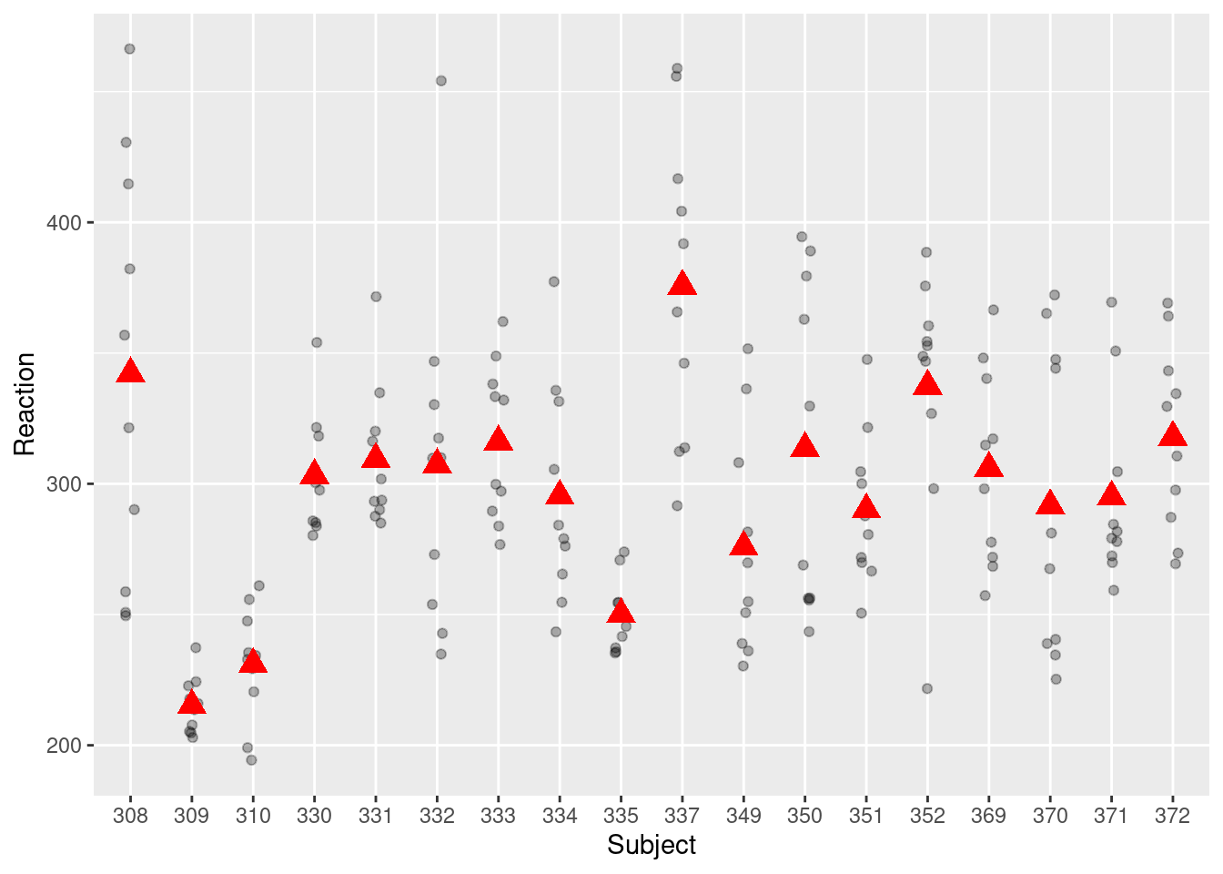
The graph below shows the distribution of the Reaction variable in the sleepstudy data.

Check your learning

What do you think is the value of ICC in the above graph?

0
0.4
0.9

Empirical Bayes Estimates

Note: OLS = ordinary least squares, the estimation method commonly used in regular regression.

Think more

When ${\sigma }^2/n_j=0$, ${\lambda }_j=1$, and the empirical Bayes estimate will be the same as the sample school mean, meaning that there is no borrowing of information. Why is there no need to borrow information in this situation?

Adding a Level-2 Predictor

Note that the ses was standardized in the data set, meaning that ses = 0 is at the sample mean, and ses = 1 means one standard deviation above the mean.

Check your learning

In regression, the independent observation assumption means that

The predictor variables should be independent
Knowing the score of one observation gives no information about other observations
The data should follow a hierarchical structure

The Design Effect

Practice yourself

Compute the design effect for mathach for the HSB data. Which of the following is the closest to your computation?

8.1
8.9
29.6
1294.1

Bonus Challenge

What is the design effect for a longitudinal study of 5 waves with 30 individuals, and an ICC for the outcome of 0.5?

1
3
15.5

Aggregation

Note

While disaggregation yields result with standard errors being too small, aggregation generally results in standard errors that are slightly larger. The main problem of aggregation, however, is that it removes all the information in the lower level, so level-1 predictors cannot be studied. MLM avoids problems of both disaggregation and aggregation.

Standard error estimates under OLS and MLM

This part is optional but gives a mathematical explanation of why OLS underestimates the standard error.

Model equations

Check your learning

In the level-2 equation with meanses as the predictor, what is the outcome variable?

student math achievement scores
school mean math achievement
variance of school means

MLM with a level-2 predictor in R

Check your learning

How do you interpret the coefficient for meanses?

The predicted difference in math achievement between two schools with one unit difference in mean SES
The mean achievement for a school with meanses = 0
The variance of math achievement accounted for by meanses

Statistical Inference

If the 95% CI excludes zero, there is evidence that the predictor has a nonzero relation with the outcome.

Check your learning

By default, what type of confidence interval is computed by the lme4 package?

Likelihood-based
Wald
Score
Bootstrap