# To install a package, run the following ONCE (and only once on your computer)
# install.packages("psych")
library(here)  # makes reading data more consistent
library(tidyverse)  # for data manipulation and plotting
library(haven)  # for importing SPSS/SAS/Stata data
library(lme4)  # for multilevel analysis
library(splines)  # for spline models
library(brms)  # for Bayesian multilevel analysis
library(modelsummary)  # for making tables
library(sjPlot) # for plotsWeek 9 (R): Longitudinal I
Load Packages and Import Data
curran_path <- here("data_files", "CurranData.sav")
if (!file.exists(curran_path)) {
    download.file(
        "https://github.com/MultiLevelAnalysis/Datasets-third-edition-Multilevel-book/raw/master/chapter%205/Curran/CurranData.sav",
        curran_path
    )
}
# Read in the data from GitHub (need Internet access)
curran_wide <- read_sav(curran_path)
# Make id a factor
curran_wide  # print the data
Wide to Long
To perform multilevel analysis, we need to restructure the data from a wide format to a long format:
# Using the new `tidyr::pivot_longer()` function
curran_long <- curran_wide %>%
    pivot_longer(
        c(anti1:anti4, read1:read4),  # variables that are repeated measures
        # Convert 8 columns to 3: 2 columns each for anti/read (.value), and
        # one column for time
        names_to = c(".value", "time"),
        # Extract the names "anti"/"read" from the names of the variables for the
        # value columns, and then the number to the "time" column
        names_pattern = "(anti|read)([1-4])",
        # Convert the "time" column to integers
        names_transform = list(time = as.integer)
    )
curran_long %>%
    select(id, anti, read, time, everything())
Data Exploration
curran_long %>%
    select(time, kidage, homecog, anti, read) %>%
    psych::pairs.panels(jiggle = TRUE, factor = 0.5, ellipses = FALSE,
                        cex.cor = 1, cex = 0.5)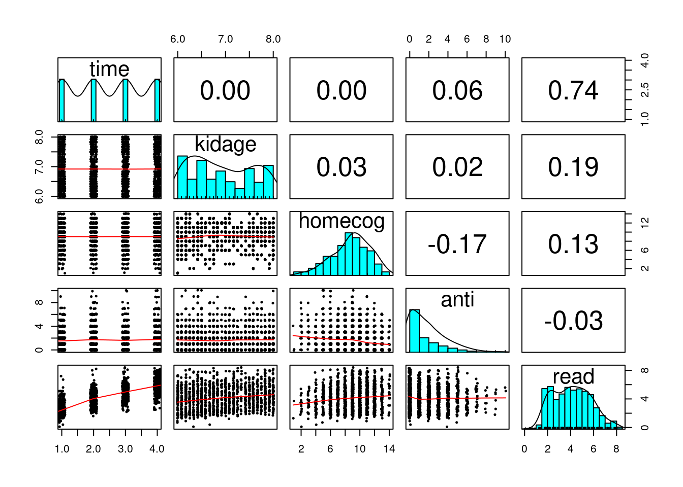
What distinguishes longitudinal data from usual cross-sectional multilevel data is the temporal ordering. In the example of students nested within schools, we don’t say that student 1 is naturally before student 2, and it doesn’t matter if one reorders the students. However, in longitudinal data, such temporal sequence is very important, and we cannot simply rearrange the observation at time 2 to be at time 1. A related concern is the presence of autocorrelation, with which observations closer in time will be more similar to each other.
Spaghetti Plot
# Plotting
p1 <- ggplot(curran_long, aes(x = time, y = read)) +
    geom_point(alpha = 0.3) +
    # add lines to connect the data for each person
    geom_line(aes(group = id), alpha = 0.3) +
    # add a mean trajectory
    stat_summary(fun = "mean", col = "red", size = 1, geom = "line")
># Warning: Using `size` aesthetic for lines was deprecated in ggplot2 3.4.0.
># ℹ Please use `linewidth` instead.p1># Warning: Removed 295 rows containing non-finite values (`stat_summary()`).># Warning: Removed 295 rows containing missing values (`geom_point()`).># Warning: Removed 250 rows containing missing values (`geom_line()`).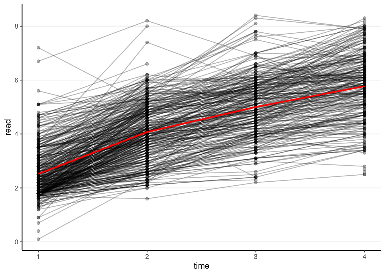
We can see that, on average, there is an increasing trend across time, but also a lot of variations in each individual’s starting point and the trajectory of change.
We can also plot the trajectory for a random sample of individuals:
# Randomly sample 40 individuals
set.seed(1349)
sampled_id <- sample(unique(curran_long$id), 40)
curran_long %>%
    filter(id %in% sampled_id) %>%
    ggplot(aes(x = time, y = read)) +
    geom_point() +
    geom_line() +  # add lines to connect the data for each person
    facet_wrap(~ id, ncol = 10)
># Warning: Removed 31 rows containing missing values (`geom_point()`).># Warning: Removed 2 rows containing missing values (`geom_line()`).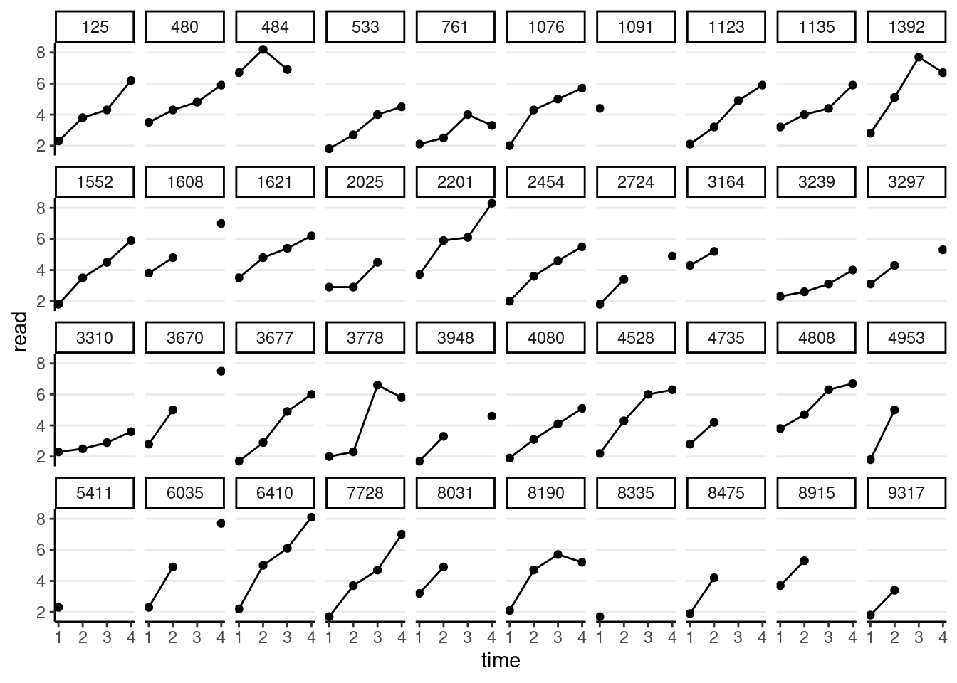
Temporal Covariances and Correlations
# Easier with the wide data set
# Covariance matrix:
curran_wide %>%
    select(starts_with("read")) %>%
    cov(use = "complete") %>%   # listwise deletion
    round(2L)  # two decimal places
># read1 read2 read3 read4
># read1 0.77 0.55 0.52 0.48
># read2 0.55 1.01 0.90 0.92
># read3 0.52 0.90 1.22 1.09
># read4 0.48 0.92 1.09 1.48# Correlation matrix
curran_wide %>%
select(starts_with("read")) %>%
cor(use = "complete") %>% # listwise deletion
round(2L) # two decimal places># read1 read2 read3 read4
># read1 1.00 0.62 0.53 0.45
># read2 0.62 1.00 0.81 0.75
># read3 0.53 0.81 1.00 0.81
># read4 0.45 0.75 0.81 1.00You can see the variances increase over time, and the correlation is generally stronger for observations closer in time.
Attrition Analyses
To see whether those who dropped out or had missing data differed in some characteristics from those who did not drop out, let’s identify the group with complete data on read, and the group without complete data on read.
# Create grouping
curran_wide <- curran_wide %>%
    # Compute summaries by rows
    rowwise() %>%
    # First compute the number of missing occasions
    mutate(nmis_read = sum(is.na(c_across(read1:read4))),
           # Complete only when nmis_read = 0
           complete = if_else(nmis_read == 0, "complete", "incomplete")) %>%
    ungroup()
# Compare the differences
datasummary((anti1 + read1 + kidgen + momage + kidage + homecog + homeemo) ~
complete * (Mean + SD), data = curran_wide)| Mean | SD | Mean | SD | |
|---|---|---|---|---|
| anti1 | 1.49 | 1.54 | 1.89 | 1.78 |
| read1 | 2.50 | 0.88 | 2.55 | 0.99 |
| gender child | 0.52 | 0.50 | 0.48 | 0.50 |
| momage | 25.61 | 1.85 | 25.42 | 1.92 |
| kidage | 6.90 | 0.62 | 6.97 | 0.66 |
| homecog | 9.09 | 2.46 | 8.63 | 2.70 |
| homeemo | 9.35 | 2.23 | 9.01 | 2.41 |
The two groups are pretty similar, except that the group with missing seems to have a higher baseline antisocial score, and lower homecog. In actual analyses, you may want to adjust for these variables by including them in the model (as covariates), if you suspect a higher probability of dropping out may confound the results.
Of course, the two groups could still be different in important characteristics that are not included in the data. It requires careful investigation of why the data were missing.
Unconditional Model
m00_lme4 <- lmer(read ~ (1 | id), data = curran_long)
summary(m00_lme4)
># Linear mixed model fit by REML ['lmerMod']
># Formula: read ~ (1 | id)
># Data: curran_long
>#
># REML criterion at convergence: 5055.9
>#
># Scaled residuals:
># Min 1Q Median 3Q Max
># -2.21699 -0.79402 0.02351 0.72466 2.34342
>#
># Random effects:
># Groups Name Variance Std.Dev.
># id (Intercept) 0.3005 0.5482
># Residual 2.3903 1.5461
># Number of obs: 1325, groups: id, 405
>#
># Fixed effects:
># Estimate Std. Error t value
># (Intercept) 4.11279 0.05093 80.75# ICC (from the performance package)
performance::icc(m00_lme4)># # Intraclass Correlation Coefficient
>#
># Adjusted ICC: 0.112
># Unadjusted ICC: 0.112However, lme4 has some limitations with longitudinal data analysis, as it assumes the so-called compound symmetry error covariance structure. Basically, that means that the within-person (level-1) error has constant variance (i.e., \(\sigma^2\)) over time, and the errors from one time point to the next are not correlated after conditioning on the fixed and random effects. In other words, whatever causes one to have a higher (or lower) score than predicted for today will not carry over to tomorrow.
There are a few more flexible packages for handling longitudinal data. You will see people use nlme a lot. glmmTMB is another option. There are also packages with Bayesian estimation, such as MCMCglmm and brms. For this class, we will use brms. Let’s replicate the results from lme4:
m00 <- brm(read ~ (1 | id), data = curran_long,
           file = "brms_cached_m00")
summary(m00)
># Family: gaussian
># Links: mu = identity; sigma = identity
># Formula: read ~ (1 | id)
># Data: curran_long (Number of observations: 1325)
># Draws: 4 chains, each with iter = 2000; warmup = 1000; thin = 1;
># total post-warmup draws = 4000
>#
># Group-Level Effects:
># ~id (Number of levels: 405)
># Estimate Est.Error l-95% CI u-95% CI Rhat Bulk_ESS Tail_ESS
># sd(Intercept) 0.54 0.08 0.38 0.68 1.00 1151 1826
>#
># Population-Level Effects:
># Estimate Est.Error l-95% CI u-95% CI Rhat Bulk_ESS Tail_ESS
># Intercept 4.11 0.05 4.01 4.21 1.00 4186 2965
>#
># Family Specific Parameters:
># Estimate Est.Error l-95% CI u-95% CI Rhat Bulk_ESS Tail_ESS
># sigma 1.55 0.04 1.48 1.63 1.00 2464 2758
>#
># Draws were sampled using sampling(NUTS). For each parameter, Bulk_ESS
># and Tail_ESS are effective sample size measures, and Rhat is the potential
># scale reduction factor on split chains (at convergence, Rhat = 1).# ICC
performance::icc(m00)># # Intraclass Correlation Coefficient
>#
># Adjusted ICC: 0.108
># Unadjusted ICC: 0.108You can see that the results are similar. The ICC values are similar too.
Unstructured Fixed Part/Compound Symmetry* (15.1.1 of Snijders & Bosker, 2012)
Instead of assuming a specific growth shape (e.g., linear), one can allow each time point to have its own mean. This provides an excellent fit to the data, but does not allow for an interpretable description of how individuals change over time, and does not test for any trends. Therefore, it is commonly used only as a reference to compare different growth models.
# Compound Symmetry (i.e., same as repeated measure ANOVA)
# Use `0 +` to suppress the intercept
m_cs_lme4 <- lmer(read ~ 0 + factor(time) + (1 | id),
             data = curran_long)
summary(m_cs_lme4)  # omnibus test for time
># Linear mixed model fit by REML ['lmerMod']
># Formula: read ~ 0 + factor(time) + (1 | id)
># Data: curran_long
>#
># REML criterion at convergence: 3375.6
>#
># Scaled residuals:
># Min 1Q Median 3Q Max
># -2.5310 -0.5345 -0.0422 0.5107 4.2102
>#
># Random effects:
># Groups Name Variance Std.Dev.
># id (Intercept) 0.7900 0.8888
># Residual 0.4075 0.6383
># Number of obs: 1325, groups: id, 405
>#
># Fixed effects:
># Estimate Std. Error t value
># factor(time)1 2.52272 0.05438 46.39
># factor(time)2 4.06800 0.05548 73.32
># factor(time)3 5.01187 0.06014 83.33
># factor(time)4 5.81222 0.06044 96.17
>#
># Correlation of Fixed Effects:
># fct()1 fct()2 fct()3
># factor(tm)2 0.647
># factor(tm)3 0.596 0.592
># factor(tm)4 0.594 0.590 0.573# This is the equivalent repeated-measure ANOVA model
# (with different estimation method)
m_rmaov <- aov(read ~ factor(time) + Error(id), data = curran_long)
summary(m_rmaov)>#
># Error: id
># Df Sum Sq Mean Sq
># factor(time) 1 4.367 4.367
>#
># Error: Within
># Df Sum Sq Mean Sq F value Pr(>F)
># factor(time) 3 1986 662.0 556.5 <2e-16 ***
># Residuals 1320 1570 1.2
># ---
># Signif. codes: 0 '***' 0.001 '**' 0.01 '*' 0.05 '.' 0.1 ' ' 1m_cs <- brm(read ~ 0 + factor(time) + (1 | id),
data = curran_long,
file = "brms_cached_m_cs"
)
summary(m_cs)># Family: gaussian
># Links: mu = identity; sigma = identity
># Formula: read ~ 0 + factor(time) + (1 | id)
># Data: curran_long (Number of observations: 1325)
># Draws: 4 chains, each with iter = 2000; warmup = 1000; thin = 1;
># total post-warmup draws = 4000
>#
># Group-Level Effects:
># ~id (Number of levels: 405)
># Estimate Est.Error l-95% CI u-95% CI Rhat Bulk_ESS Tail_ESS
># sd(Intercept) 0.89 0.04 0.82 0.96 1.00 1092 1841
>#
># Population-Level Effects:
># Estimate Est.Error l-95% CI u-95% CI Rhat Bulk_ESS Tail_ESS
># factortime1 2.52 0.05 2.42 2.63 1.01 631 1369
># factortime2 4.07 0.05 3.96 4.18 1.01 590 1718
># factortime3 5.01 0.06 4.89 5.13 1.00 763 1782
># factortime4 5.81 0.06 5.69 5.93 1.01 716 1921
>#
># Family Specific Parameters:
># Estimate Est.Error l-95% CI u-95% CI Rhat Bulk_ESS Tail_ESS
># sigma 0.64 0.01 0.61 0.67 1.00 3051 2503
>#
># Draws were sampled using sampling(NUTS). For each parameter, Bulk_ESS
># and Tail_ESS are effective sample size measures, and Rhat is the potential
># scale reduction factor on split chains (at convergence, Rhat = 1).From this model, you can compute the conditional ICC, which is the proportion of between-person variance out of the total variance in the detrended data.
# "Adjusted ICC" = Conditional ICC
performance::icc(m_cs)
># # Intraclass Correlation Coefficient
>#
># Adjusted ICC: 0.660
># Unadjusted ICC: 0.291So after removing the trend, the between-person variance is larger than the within-person variance.
Linear Growth Models
Linear Model With Time
Level 1: Within-Person
\[\text{read}_{ti} = \beta_{0i} + \beta_{1i} \text{time}_{ti} + e_{ti}\]
Level 2: Between-Person
\[ \begin{aligned} \beta_{0i} = \gamma_{00} + u_{0i} \\ \beta_{1i} = \gamma_{10} + u_{1i} \end{aligned} \]
# Fit a linear growth model with no random slopes (not commonly done)
m_gca_lme4 <- lmer(read ~ time0 + (time0 | id), data = curran_long)
summary(m_gca_lme4)
># Linear mixed model fit by REML ['lmerMod']
># Formula: read ~ time0 + (time0 | id)
># Data: curran_long
>#
># REML criterion at convergence: 3382
>#
># Scaled residuals:
># Min 1Q Median 3Q Max
># -2.7161 -0.5201 -0.0220 0.4793 4.1847
>#
># Random effects:
># Groups Name Variance Std.Dev. Corr
># id (Intercept) 0.57309 0.7570
># time0 0.07459 0.2731 0.29
># Residual 0.34584 0.5881
># Number of obs: 1325, groups: id, 405
>#
># Fixed effects:
># Estimate Std. Error t value
># (Intercept) 2.69609 0.04530 59.52
># time0 1.11915 0.02169 51.60
>#
># Correlation of Fixed Effects:
># (Intr)
># time0 -0.155random_persons <- sample(unique(curran_long$id), size = 24)
broom.mixed::augment(m_gca_lme4) %>%
# Select only the 24 participants
filter(id %in% random_persons) %>%
ggplot(aes(x = time0, y = read)) +
geom_point() +
geom_line(aes(y = .fitted), col = "blue") +
facet_wrap(~ id, ncol = 6)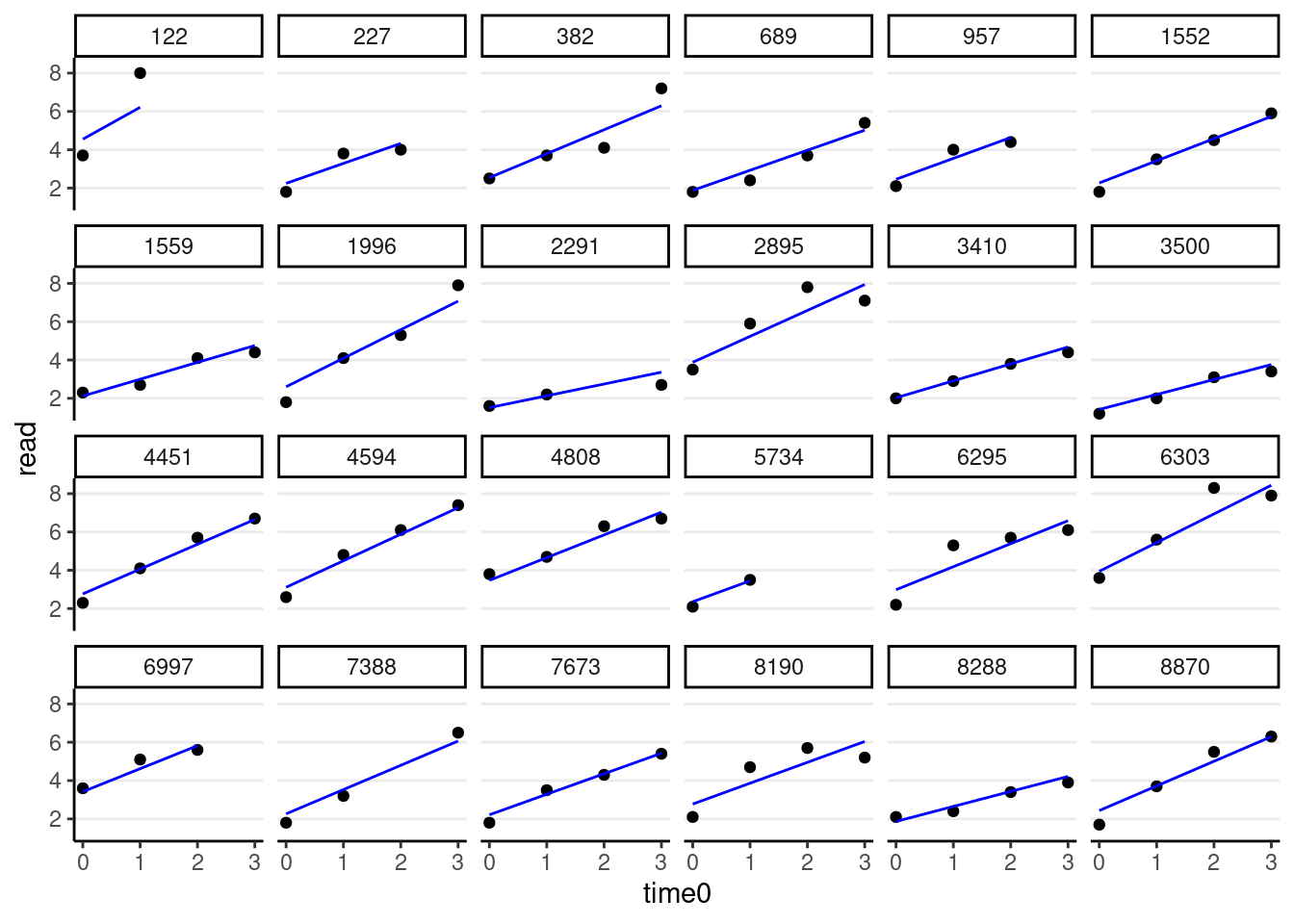
# Fit a linear growth model with no random slopes (not commonly done)
m_gca <- brm(read ~ time0 + (time0 | id), data = curran_long,
             file = "brms_cached_m_gca")
summary(m_gca)
># Family: gaussian
># Links: mu = identity; sigma = identity
># Formula: read ~ time0 + (time0 | id)
># Data: curran_long (Number of observations: 1325)
># Draws: 4 chains, each with iter = 2000; warmup = 1000; thin = 1;
># total post-warmup draws = 4000
>#
># Group-Level Effects:
># ~id (Number of levels: 405)
># Estimate Est.Error l-95% CI u-95% CI Rhat Bulk_ESS
># sd(Intercept) 0.76 0.04 0.68 0.84 1.00 1501
># sd(time0) 0.27 0.02 0.22 0.32 1.00 834
># cor(Intercept,time0) 0.30 0.12 0.08 0.53 1.00 872
># Tail_ESS
># sd(Intercept) 2356
># sd(time0) 1698
># cor(Intercept,time0) 1246
>#
># Population-Level Effects:
># Estimate Est.Error l-95% CI u-95% CI Rhat Bulk_ESS Tail_ESS
># Intercept 2.70 0.04 2.61 2.78 1.00 2141 3057
># time0 1.12 0.02 1.08 1.16 1.00 3660 2965
>#
># Family Specific Parameters:
># Estimate Est.Error l-95% CI u-95% CI Rhat Bulk_ESS Tail_ESS
># sigma 0.59 0.02 0.56 0.63 1.00 1157 2200
>#
># Draws were sampled using sampling(NUTS). For each parameter, Bulk_ESS
># and Tail_ESS are effective sample size measures, and Rhat is the potential
># scale reduction factor on split chains (at convergence, Rhat = 1).random_persons <- sample(unique(curran_long$id), size = 24)
broom.mixed::augment(m_gca) %>%
# Select only the 24 participants
filter(id %in% random_persons) %>%
ggplot(aes(x = time0, y = read)) +
geom_point() +
# Add 95% confidence band
geom_ribbon(aes(ymin = .fitted - 2 * .se.fit,
ymax = .fitted + 2 * .se.fit),
alpha = 0.1) +
geom_line(aes(y = .fitted), col = "blue") +
facet_wrap(~ id, ncol = 6)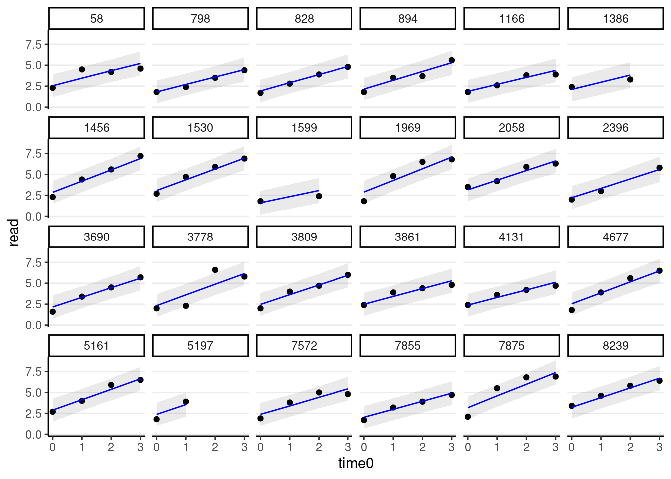
Piecewise Growth Model
A piecewise linear growth assumes two or more phases of linear change across time. For example, we can assume that, for our data, phase 1 is from Time 0 to Time 1, and phase 2 is from Time 1 to Time 3.
Because we’re estimating two slopes, we need two predictors: phase1 represents the initial slope from Time 0 to Time 1, and phase2 represents the slope from Time 1 to Time 3. The coding is shown below:
\[\begin{bmatrix} \textrm{phase1} & \textrm{phase2} \\ 0 & 0 \\ 1 & 0 \\ 1 & 1 \\ 1 & 2 \end{bmatrix}\]
To understand the coding, in phase1 the line changes from Time 0 to Time 1, but stays there. phase2 has 0 from Time 0 to Time 1 as nothing should have happened. Then, From Time 1 to Time 3, it starts to increase linearly.
One way to check whether you’ve specified the coding correctly is to sum the numbers in every row, which you should get back 0, 1, 2, 3, . . .
Below is an example where intercept = 1, growth in phase 1 = 0.5, growth in phase 2 = 0.8. The dashed line shows the contribution from phase1 (plus the intercept). The red dotted line shows the contribution from phase2.
demo_df <- tibble(TIME = c(0, 1, 2, 3))
ggplot(demo_df, aes(x = TIME)) +
    stat_function(fun = function(x) 1 + 0.5 * pmin(x, 1),
                  linetype = "dashed", size = 1.5) +
    stat_function(fun = function(x) 0.8 * pmax(x - 1, 0), col = "red",
                  linetype = "dotted", size = 1.5) +
    stat_function(fun = function(x) 1 + 0.5 * pmin(x, 1) + 0.8 * pmax(x - 1, 0))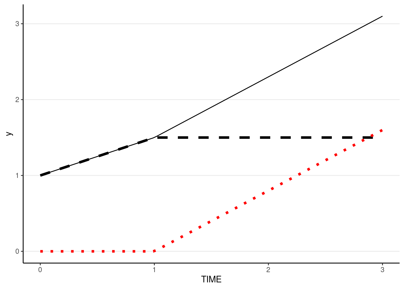
Now, we assume Time 0 to Time 1 has one slope, and Time 1 to Time 3 has another slope.
# Compute phase1 and phase2
curran_long <- curran_long %>%
    mutate(phase1 = pmin(time0, 1),  # anything bigger than 1 becomes 1
           phase2 = pmax(time0 - 1, 0))  # set time to start at TIME 1, and then make
# anything smaller than 0 to 0
# Check the coding:
curran_long %>%
    select(time0, phase1, phase2) %>%
    distinct()
We can define a function piece() that gives us the coding to be used in the model formula:
piece <- function(x, node) {
    cbind(pmin(x, node),
          pmax(x - node, 0))
}# Fit the piecewise growth model
m_pw_lme4 <- lmer(read ~ piece(time0, node = 1) +
(piece(time0, node = 1) | id),
data = curran_long)># boundary (singular) fit: see help('isSingular')summary(m_pw_lme4)># Linear mixed model fit by REML ['lmerMod']
># Formula: read ~ piece(time0, node = 1) + (piece(time0, node = 1) | id)
># Data: curran_long
>#
># REML criterion at convergence: 3209.7
>#
># Scaled residuals:
># Min 1Q Median 3Q Max
># -3.1392 -0.4559 -0.0315 0.4013 4.2351
>#
># Random effects:
># Groups Name Variance Std.Dev. Corr
># id (Intercept) 0.60514 0.7779
># piece(time0, node = 1)1 0.22641 0.4758 0.13
># piece(time0, node = 1)2 0.05362 0.2316 -0.15 0.96
># Residual 0.25156 0.5016
># Number of obs: 1325, groups: id, 405
>#
># Fixed effects:
># Estimate Std. Error t value
># (Intercept) 2.52272 0.04599 54.85
># piece(time0, node = 1)1 1.56213 0.04269 36.60
># piece(time0, node = 1)2 0.87936 0.02544 34.57
>#
># Correlation of Fixed Effects:
># (Intr) p(0,n=1)1
># pc(t0,n=1)1 -0.256
># pc(t0,n=1)2 -0.058 -0.077
># optimizer (nloptwrap) convergence code: 0 (OK)
># boundary (singular) fit: see help('isSingular')# Fit the piecewise growth model (using the `I()` syntax)
# for easier plotting
m_pw <- brm(
read ~ piece(time0, node = 1) + (piece(time0, node = 1) | id),
data = curran_long,
file = "brms_cached_m_pw",
# increase adapt_delta as there was a divergent transition warning
control = list(adapt_delta = 0.9)
)
summary(m_pw)># Family: gaussian
># Links: mu = identity; sigma = identity
># Formula: read ~ piece(time0, node = 1) + (piece(time0, node = 1) | id)
># Data: curran_long (Number of observations: 1325)
># Draws: 4 chains, each with iter = 2000; warmup = 1000; thin = 1;
># total post-warmup draws = 4000
>#
># Group-Level Effects:
># ~id (Number of levels: 405)
># Estimate Est.Error l-95% CI u-95% CI
># sd(Intercept) 0.78 0.04 0.71 0.86
># sd(piecetime0nodeEQ11) 0.50 0.05 0.40 0.60
># sd(piecetime0nodeEQ12) 0.24 0.03 0.18 0.31
># cor(Intercept,piecetime0nodeEQ11) 0.11 0.11 -0.10 0.35
># cor(Intercept,piecetime0nodeEQ12) -0.11 0.13 -0.35 0.14
># cor(piecetime0nodeEQ11,piecetime0nodeEQ12) 0.77 0.15 0.43 0.98
># Rhat Bulk_ESS Tail_ESS
># sd(Intercept) 1.00 1441 2788
># sd(piecetime0nodeEQ11) 1.00 1137 1905
># sd(piecetime0nodeEQ12) 1.00 1092 2149
># cor(Intercept,piecetime0nodeEQ11) 1.00 1446 2380
># cor(Intercept,piecetime0nodeEQ12) 1.00 2385 3090
># cor(piecetime0nodeEQ11,piecetime0nodeEQ12) 1.00 573 1216
>#
># Population-Level Effects:
># Estimate Est.Error l-95% CI u-95% CI Rhat Bulk_ESS Tail_ESS
># Intercept 2.52 0.05 2.43 2.62 1.00 2193 2767
># piecetime0nodeEQ11 1.56 0.04 1.48 1.65 1.00 4774 3531
># piecetime0nodeEQ12 0.88 0.03 0.83 0.93 1.00 5974 3254
>#
># Family Specific Parameters:
># Estimate Est.Error l-95% CI u-95% CI Rhat Bulk_ESS Tail_ESS
># sigma 0.50 0.02 0.47 0.53 1.00 836 1369
>#
># Draws were sampled using sampling(NUTS). For each parameter, Bulk_ESS
># and Tail_ESS are effective sample size measures, and Rhat is the potential
># scale reduction factor on split chains (at convergence, Rhat = 1).The piecewise model is actually equivalent to the linear spline model, although it is parameterized differently.
# Fit the piecewise growth model (use `splines::bs()`)
m_lin_spline <- brm(
    read ~ bs(time0, knots = 1, degree = 1) +
        (bs(time0, knots = 1, degree = 1) | id),
    data = curran_long,
    file = "brms_cached_m_lin_spline",
    # increase adapt_delta as there was a divergent transition warning
    control = list(adapt_delta = 0.9)
)
summary(m_lin_spline)
># Family: gaussian
># Links: mu = identity; sigma = identity
># Formula: read ~ bs(time0, knots = 1, degree = 1) + (bs(time0, knots = 1, degree = 1) | id)
># Data: curran_long (Number of observations: 1325)
># Draws: 4 chains, each with iter = 2000; warmup = 1000; thin = 1;
># total post-warmup draws = 4000
>#
># Group-Level Effects:
># ~id (Number of levels: 405)
># Estimate Est.Error
># sd(Intercept) 0.78 0.04
># sd(bstime0knotsEQ1degreeEQ11) 0.49 0.05
># sd(bstime0knotsEQ1degreeEQ12) 0.93 0.06
># cor(Intercept,bstime0knotsEQ1degreeEQ11) 0.12 0.12
># cor(Intercept,bstime0knotsEQ1degreeEQ12) -0.00 0.09
># cor(bstime0knotsEQ1degreeEQ11,bstime0knotsEQ1degreeEQ12) 0.93 0.05
># l-95% CI u-95% CI Rhat
># sd(Intercept) 0.71 0.87 1.00
># sd(bstime0knotsEQ1degreeEQ11) 0.39 0.59 1.01
># sd(bstime0knotsEQ1degreeEQ12) 0.81 1.05 1.00
># cor(Intercept,bstime0knotsEQ1degreeEQ11) -0.09 0.35 1.00
># cor(Intercept,bstime0knotsEQ1degreeEQ12) -0.17 0.18 1.00
># cor(bstime0knotsEQ1degreeEQ11,bstime0knotsEQ1degreeEQ12) 0.81 0.99 1.01
># Bulk_ESS Tail_ESS
># sd(Intercept) 1541 2544
># sd(bstime0knotsEQ1degreeEQ11) 841 1859
># sd(bstime0knotsEQ1degreeEQ12) 1120 1953
># cor(Intercept,bstime0knotsEQ1degreeEQ11) 1150 2110
># cor(Intercept,bstime0knotsEQ1degreeEQ12) 1121 2056
># cor(bstime0knotsEQ1degreeEQ11,bstime0knotsEQ1degreeEQ12) 455 1198
>#
># Population-Level Effects:
># Estimate Est.Error l-95% CI u-95% CI Rhat Bulk_ESS
># Intercept 2.52 0.05 2.43 2.61 1.00 2180
># bstime0knotsEQ1degreeEQ11 1.56 0.04 1.48 1.65 1.00 3102
># bstime0knotsEQ1degreeEQ12 3.32 0.06 3.20 3.45 1.00 2642
># Tail_ESS
># Intercept 2493
># bstime0knotsEQ1degreeEQ11 3251
># bstime0knotsEQ1degreeEQ12 2878
>#
># Family Specific Parameters:
># Estimate Est.Error l-95% CI u-95% CI Rhat Bulk_ESS Tail_ESS
># sigma 0.50 0.02 0.46 0.53 1.01 629 1490
>#
># Draws were sampled using sampling(NUTS). For each parameter, Bulk_ESS
># and Tail_ESS are effective sample size measures, and Rhat is the potential
># scale reduction factor on split chains (at convergence, Rhat = 1).Plotting the predicted trajectories
Average predicted trajectory
plot_model(m_pw, type = "pred", show.data = TRUE, jitter = 0.05)># Note: uncertainty of error terms are not taken into account. You may want to use `rstantools::posterior_predict()`.># $time0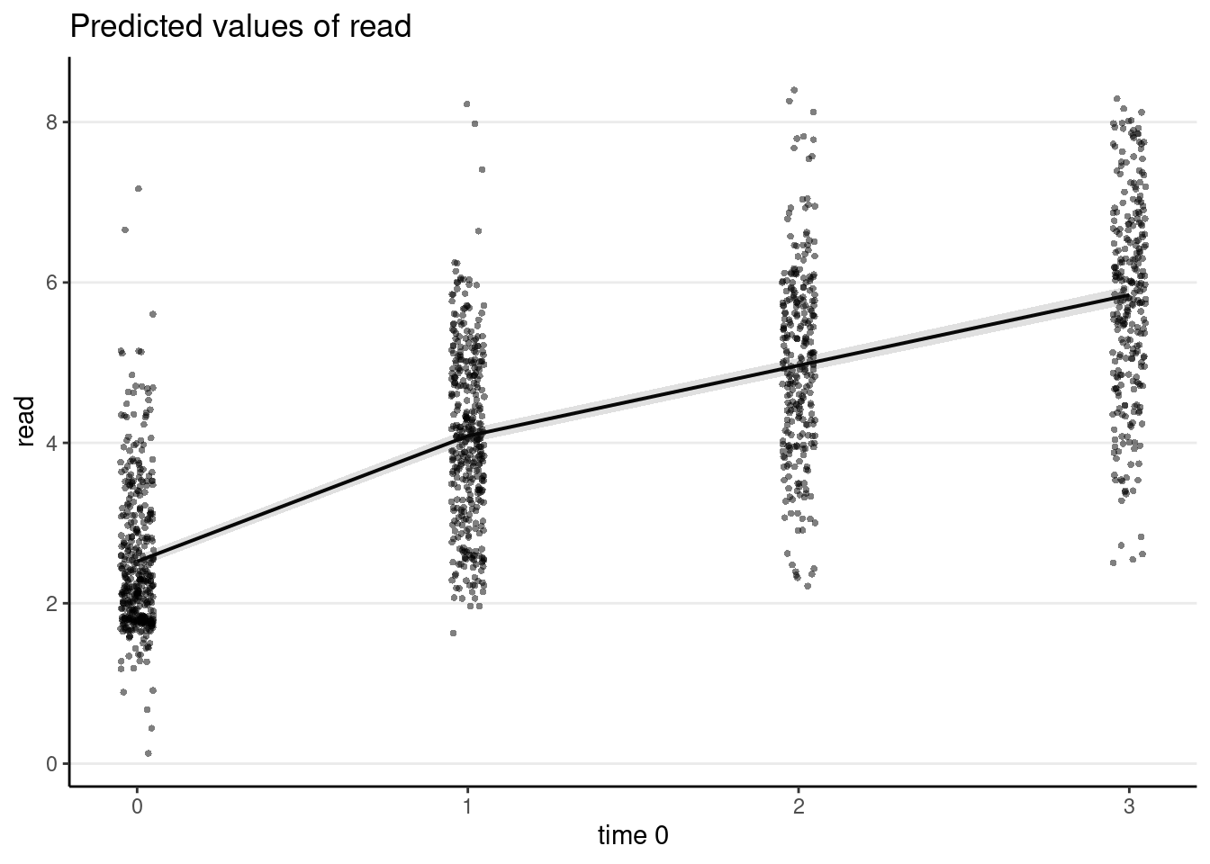
Predicted trajectories at the individual level
# Add predicted lines to individual trajectories
broom.mixed::augment(m_pw) %>%
    # Select only the 24 participants
    filter(id %in% random_persons) %>%
    ggplot(aes(x = time0, y = read)) +
    geom_point() +
    # Add 95% confidence band
    geom_ribbon(aes(ymin = .fitted - 2 * .se.fit,
                    ymax = .fitted + 2 * .se.fit),
                alpha = 0.1) +
    geom_line(aes(y = .fitted), col = "blue") +
    facet_wrap(~ id, ncol = 6)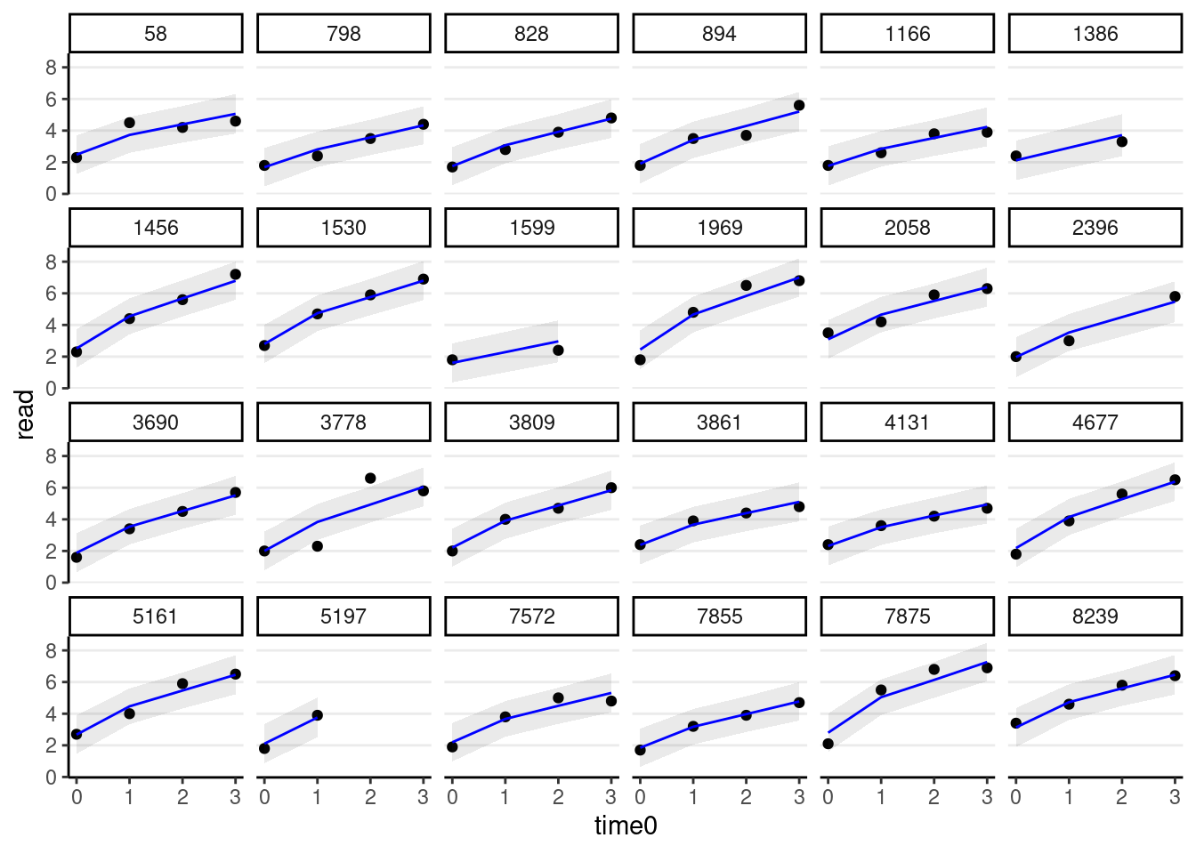
Model Comparison
One way to compare different models with the same outcome variable and the same data set is to use some kind of information criterion. The most well-known one is the Akaike information criterion. A model with a lower AIC is expected to better predict future observations similar to the current sample. For example,
AIC(m_gca_lme4, m_pw_lme4)The analog with Bayesian estimation is the **leave-one-out (LOO) criterion:
loo(m_gca, m_pw)># Warning: Found 103 observations with a pareto_k > 0.7 in model 'm_gca'. It is
># recommended to set 'moment_match = TRUE' in order to perform moment matching for
># problematic observations.># Warning: Found 186 observations with a pareto_k > 0.7 in model 'm_pw'. It is
># recommended to set 'moment_match = TRUE' in order to perform moment matching for
># problematic observations.># Output of model 'm_gca':
>#
># Computed from 4000 by 1325 log-likelihood matrix
>#
># Estimate SE
># elpd_loo -1476.9 33.6
># p_loo 439.7 17.7
># looic 2953.8 67.1
># ------
># Monte Carlo SE of elpd_loo is NA.
>#
># Pareto k diagnostic values:
># Count Pct. Min. n_eff
># (-Inf, 0.5] (good) 894 67.5% 346
># (0.5, 0.7] (ok) 328 24.8% 66
># (0.7, 1] (bad) 100 7.5% 17
># (1, Inf) (very bad) 3 0.2% 2
># See help('pareto-k-diagnostic') for details.
>#
># Output of model 'm_pw':
>#
># Computed from 4000 by 1325 log-likelihood matrix
>#
># Estimate SE
># elpd_loo -1329.0 35.1
># p_loo 533.8 20.9
># looic 2658.1 70.3
># ------
># Monte Carlo SE of elpd_loo is NA.
>#
># Pareto k diagnostic values:
># Count Pct. Min. n_eff
># (-Inf, 0.5] (good) 671 50.6% 364
># (0.5, 0.7] (ok) 468 35.3% 87
># (0.7, 1] (bad) 172 13.0% 13
># (1, Inf) (very bad) 14 1.1% 3
># See help('pareto-k-diagnostic') for details.
>#
># Model comparisons:
># elpd_diff se_diff
># m_pw 0.0 0.0
># m_gca -147.8 15.3The model with a lower AIC/LOOIC should be preferred. In this case, the piecewise model is better.
Time-Invariant Covariates
Time-invariant covariate = Another way to say a level-2 variable.
You can add homecog and its interaction to the model with age as predictors. Now there are two interaction terms: one with the first piece and the other with the second piece.
# Add `homecog` and its interaction with growth
# First, center homecog to 9
curran_long$homecog9 <- curran_long$homecog - 9
m_pw_homecog <- brm(
    read ~ piece(time0, node = 1) * homecog9 +
      (piece(time0, node = 1) | id),
    data = curran_long,
    file = "brms_cached_m_pw_homecog",
    # increase adapt_delta as there was a divergent transition warning
    control = list(adapt_delta = 0.9)
)
summary(m_pw_homecog)
># Family: gaussian
># Links: mu = identity; sigma = identity
># Formula: read ~ piece(time0, node = 1) * homecog9 + (piece(time0, node = 1) | id)
># Data: curran_long (Number of observations: 1325)
># Draws: 4 chains, each with iter = 2000; warmup = 1000; thin = 1;
># total post-warmup draws = 4000
>#
># Group-Level Effects:
># ~id (Number of levels: 405)
># Estimate Est.Error l-95% CI u-95% CI
># sd(Intercept) 0.78 0.04 0.70 0.86
># sd(piecetime0nodeEQ11) 0.49 0.05 0.38 0.59
># sd(piecetime0nodeEQ12) 0.24 0.03 0.18 0.31
># cor(Intercept,piecetime0nodeEQ11) 0.08 0.12 -0.13 0.34
># cor(Intercept,piecetime0nodeEQ12) -0.13 0.13 -0.36 0.13
># cor(piecetime0nodeEQ11,piecetime0nodeEQ12) 0.76 0.15 0.41 0.97
># Rhat Bulk_ESS Tail_ESS
># sd(Intercept) 1.00 1649 2698
># sd(piecetime0nodeEQ11) 1.01 991 2004
># sd(piecetime0nodeEQ12) 1.00 677 1403
># cor(Intercept,piecetime0nodeEQ11) 1.00 1481 1997
># cor(Intercept,piecetime0nodeEQ12) 1.00 2237 2853
># cor(piecetime0nodeEQ11,piecetime0nodeEQ12) 1.01 398 804
>#
># Population-Level Effects:
># Estimate Est.Error l-95% CI u-95% CI Rhat Bulk_ESS
># Intercept 2.53 0.05 2.43 2.62 1.00 2040
># piecetime0nodeEQ11 1.57 0.04 1.48 1.65 1.00 4003
># piecetime0nodeEQ12 0.88 0.03 0.83 0.93 1.00 4630
># homecog9 0.04 0.02 0.01 0.08 1.00 1927
># piecetime0nodeEQ11:homecog9 0.04 0.02 0.01 0.08 1.00 4493
># piecetime0nodeEQ12:homecog9 0.01 0.01 -0.01 0.03 1.00 4962
># Tail_ESS
># Intercept 2463
># piecetime0nodeEQ11 3304
># piecetime0nodeEQ12 3273
># homecog9 2388
># piecetime0nodeEQ11:homecog9 2689
># piecetime0nodeEQ12:homecog9 2970
>#
># Family Specific Parameters:
># Estimate Est.Error l-95% CI u-95% CI Rhat Bulk_ESS Tail_ESS
># sigma 0.50 0.02 0.47 0.53 1.00 758 1397
>#
># Draws were sampled using sampling(NUTS). For each parameter, Bulk_ESS
># and Tail_ESS are effective sample size measures, and Rhat is the potential
># scale reduction factor on split chains (at convergence, Rhat = 1).# `conditional_effects` only works for brms objects
plot(
conditional_effects(
m_pw_homecog,
effects = "time0:homecog9"
),
points = TRUE,
point_args = list(width = 0.05, alpha = 0.3)
)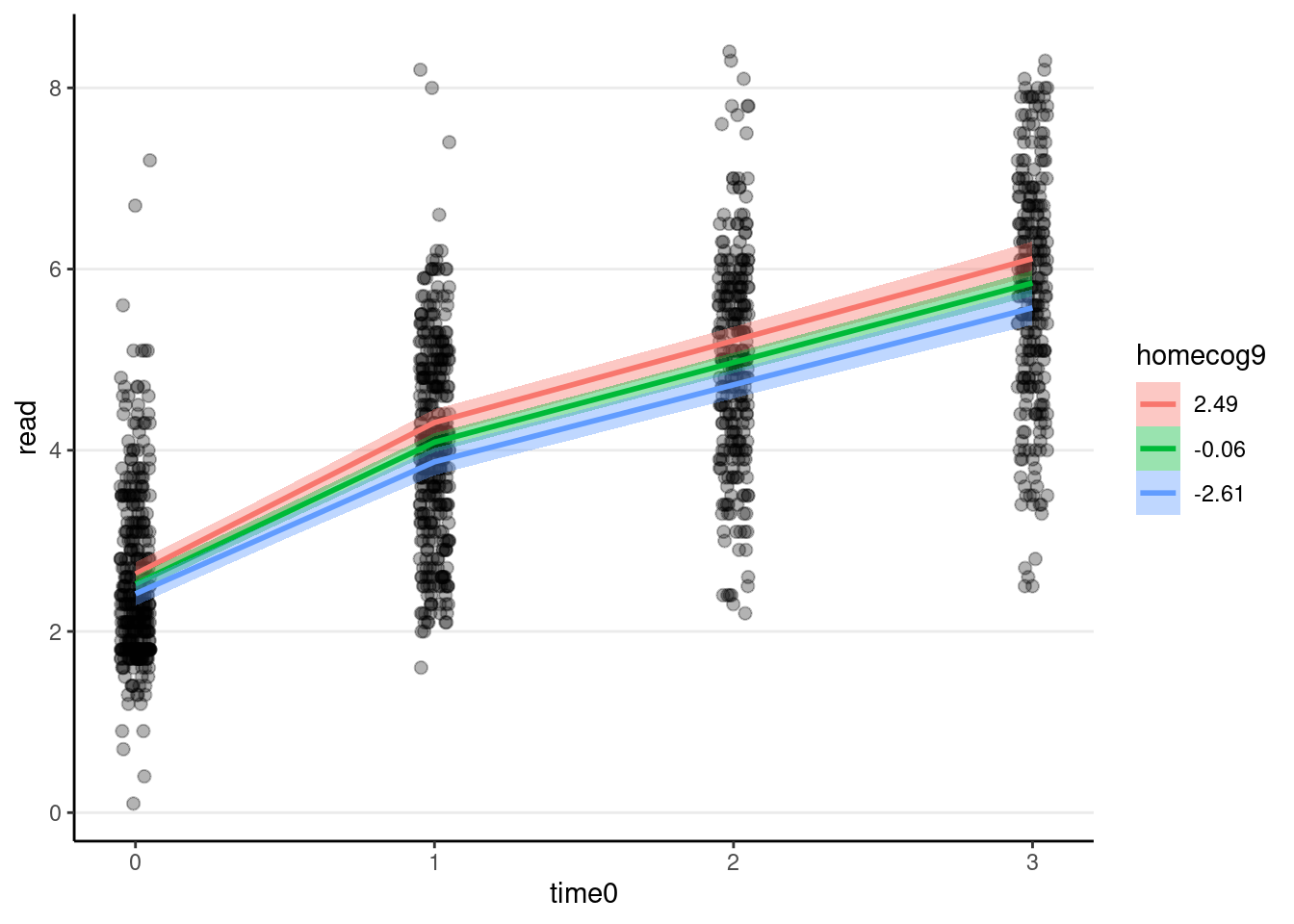
Table of Coefficients
msummary(
    list(
        "Compound Symmetry" = m00,
        "GCA" = m_gca,
        "Piecewise" = m_pw,
        "Piecewise + homecog" = m_pw_homecog
    ),
    statistic = "[{conf.low}, {conf.high}]",
    shape = effect + term ~ model,
    gof_map = c("nobs", "looic"),
    metrics = "LOOIC"
)| Compound Symmetry | GCA | Piecewise | Piecewise + homecog | ||
|---|---|---|---|---|---|
| fixed | b_Intercept | 4.113 | 2.696 | 2.522 | 2.527 |
| [4.014, 4.213] | [2.607, 2.782] | [2.431, 2.616] | [2.434, 2.620] | ||
| sigma | 1.550 | 0.590 | 0.499 | 0.499 | |
| [1.482, 1.627] | [0.559, 0.626] | [0.467, 0.532] | [0.466, 0.534] | ||
| b_time0 | 1.119 | ||||
| [1.076, 1.163] | |||||
| b_piecetime0nodeEQ11 | 1.563 | 1.568 | |||
| [1.479, 1.648] | [1.480, 1.648] | ||||
| b_piecetime0nodeEQ12 | 0.879 | 0.880 | |||
| [0.831, 0.930] | [0.829, 0.931] | ||||
| b_homecog9 | 0.043 | ||||
| [0.007, 0.079] | |||||
| b_piecetime0nodeEQ11 × homecog9 | 0.042 | ||||
| [0.008, 0.076] | |||||
| b_piecetime0nodeEQ12 × homecog9 | 0.010 | ||||
| [−0.009, 0.032] | |||||
| random | sd_id__Intercept | 0.542 | 0.756 | 0.782 | 0.776 |
| [0.379, 0.681] | [0.682, 0.837] | [0.709, 0.862] | [0.698, 0.858] | ||
| sd_id__time0 | 0.272 | ||||
| [0.225, 0.322] | |||||
| cor_id__Intercept__time0 | 0.292 | ||||
| [0.076, 0.535] | |||||
| sd_id__piecetime0nodeEQ11 | 0.496 | 0.486 | |||
| [0.397, 0.598] | [0.383, 0.587] | ||||
| sd_id__piecetime0nodeEQ12 | 0.244 | 0.243 | |||
| [0.183, 0.310] | [0.184, 0.309] | ||||
| cor_id__Intercept__piecetime0nodeEQ11 | 0.106 | 0.076 | |||
| [−0.104, 0.349] | [−0.127, 0.337] | ||||
| cor_id__Intercept__piecetime0nodeEQ12 | −0.115 | −0.136 | |||
| [−0.352, 0.142] | [−0.364, 0.131] | ||||
| cor_id__piecetime0nodeEQ11__piecetime0nodeEQ12 | 0.797 | 0.790 | |||
| [0.428, 0.975] | [0.406, 0.973] | ||||
| Num.Obs. | 1325 | 1325 | 1325 | 1325 | |
| LOOIC | 5042.2 | 2953.8 | 2658.1 | 2660.8 |
Varying Occasions
MLM can handle varying measurement occasions. For example, maybe some students are first measured in September when the semester starts, whereas others are first measured in October or November. How important this difference is depends on the research being studied. For especially infant/early childhood research, one month can already mean a lot of growth, so it is important to consider that.
Instead of using time, one can instead model an outcome variable as a function of age, with the kidage variable. To use age, however, one may want the intercept to be at a specific age, not age = 0. In the data set, the minimum age is 6. Therefore, we can subtract 6 from the original kidage variable, so that the zero point represent someone at age = 6.
Quadratic Function
Here is an example:
# Subtract age by 6
curran_long <- curran_long %>%
    mutate(kidagetv = kidage + time * 2,
           # Compute the age for each time point
           kidage6tv = kidagetv - 6)
# Plot the data
ggplot(curran_long, aes(x = kidage6tv, y = read)) +
    geom_point(size = 0.5) +
    # add lines to connect the data for each person
    geom_line(aes(group = id), alpha = 0.5) +
    # add a mean trajectory
    geom_smooth(col = "red", size = 1)
># `geom_smooth()` using method = 'gam' and formula = 'y ~ s(x, bs = "cs")'># Warning: Removed 295 rows containing non-finite values (`stat_smooth()`).># Warning: Removed 295 rows containing missing values (`geom_point()`).># Warning: Removed 250 rows containing missing values (`geom_line()`).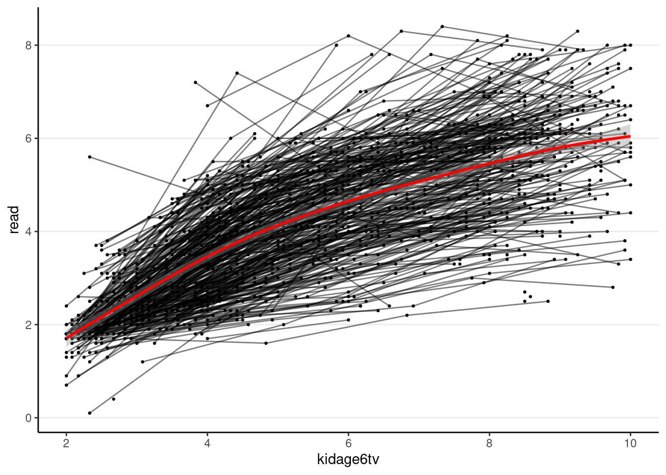
# Fit a quadratic model
m_agesq <- brm(
    read ~ kidage6tv + I(kidage6tv^2) + (kidage6tv + I(kidage6tv^2) | id),
    data = curran_long,
    file = "brms_cached_m_agesq",
    # increase adapt_delta as there was a divergent transition warning
    control = list(adapt_delta = 0.9)
)
summary(m_agesq)
># Warning: Parts of the model have not converged (some Rhats are > 1.05). Be
># careful when analysing the results! We recommend running more iterations and/or
># setting stronger priors.># Family: gaussian
># Links: mu = identity; sigma = identity
># Formula: read ~ kidage6tv + I(kidage6tv^2) + (kidage6tv + I(kidage6tv^2) | id)
># Data: curran_long (Number of observations: 1325)
># Draws: 4 chains, each with iter = 2000; warmup = 1000; thin = 1;
># total post-warmup draws = 4000
>#
># Group-Level Effects:
># ~id (Number of levels: 405)
># Estimate Est.Error l-95% CI u-95% CI Rhat Bulk_ESS
># sd(Intercept) 0.51 0.12 0.26 0.75 1.00 1189
># sd(kidage6tv) 0.40 0.05 0.30 0.50 1.01 561
># sd(Ikidage6tvE2) 0.03 0.00 0.02 0.04 1.02 298
># cor(Intercept,kidage6tv) -0.90 0.08 -0.99 -0.72 1.08 40
># cor(Intercept,Ikidage6tvE2) 0.79 0.14 0.47 0.96 1.05 69
># cor(kidage6tv,Ikidage6tvE2) -0.95 0.02 -0.98 -0.90 1.00 1318
># Tail_ESS
># sd(Intercept) 1325
># sd(kidage6tv) 795
># sd(Ikidage6tvE2) 580
># cor(Intercept,kidage6tv) 161
># cor(Intercept,Ikidage6tvE2) 208
># cor(kidage6tv,Ikidage6tvE2) 1247
>#
># Population-Level Effects:
># Estimate Est.Error l-95% CI u-95% CI Rhat Bulk_ESS Tail_ESS
># Intercept -0.32 0.10 -0.51 -0.13 1.00 4104 3489
># kidage6tv 1.13 0.04 1.04 1.21 1.00 2723 2724
># Ikidage6tvE2 -0.05 0.00 -0.06 -0.04 1.00 3203 2785
>#
># Family Specific Parameters:
># Estimate Est.Error l-95% CI u-95% CI Rhat Bulk_ESS Tail_ESS
># sigma 0.50 0.01 0.47 0.53 1.00 1241 1866
>#
># Draws were sampled using sampling(NUTS). For each parameter, Bulk_ESS
># and Tail_ESS are effective sample size measures, and Rhat is the potential
># scale reduction factor on split chains (at convergence, Rhat = 1).You can then perform the diagnostics and see whether the individual growth shape appears quadratic.
random_persons <- sample(unique(curran_long$id), size = 24)
broom.mixed::augment(m_agesq) %>%
    # Select only the 24 participants
    filter(id %in% random_persons) %>%
    ggplot(aes(x = kidage6tv, y = read)) +
    geom_point() +
    # Add 95% confidence band
    geom_ribbon(aes(ymin = .fitted - 2 * .se.fit,
                    ymax = .fitted + 2 * .se.fit),
                alpha = 0.1) +
    geom_line(aes(y = .fitted), col = "blue") +
    facet_wrap(~ id, ncol = 6)
># `geom_line()`: Each group consists of only one observation.
># ℹ Do you need to adjust the group aesthetic?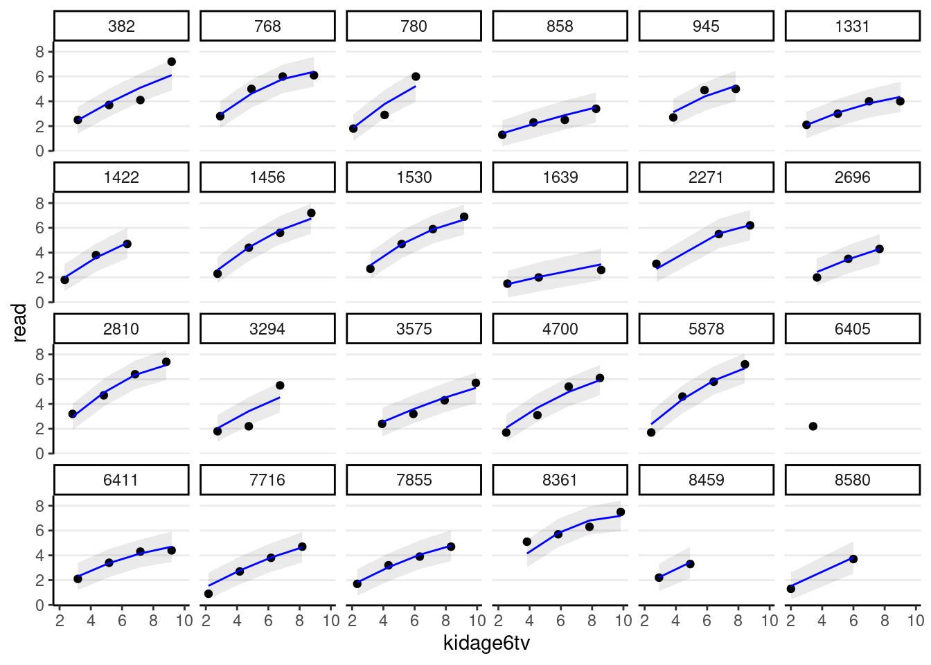
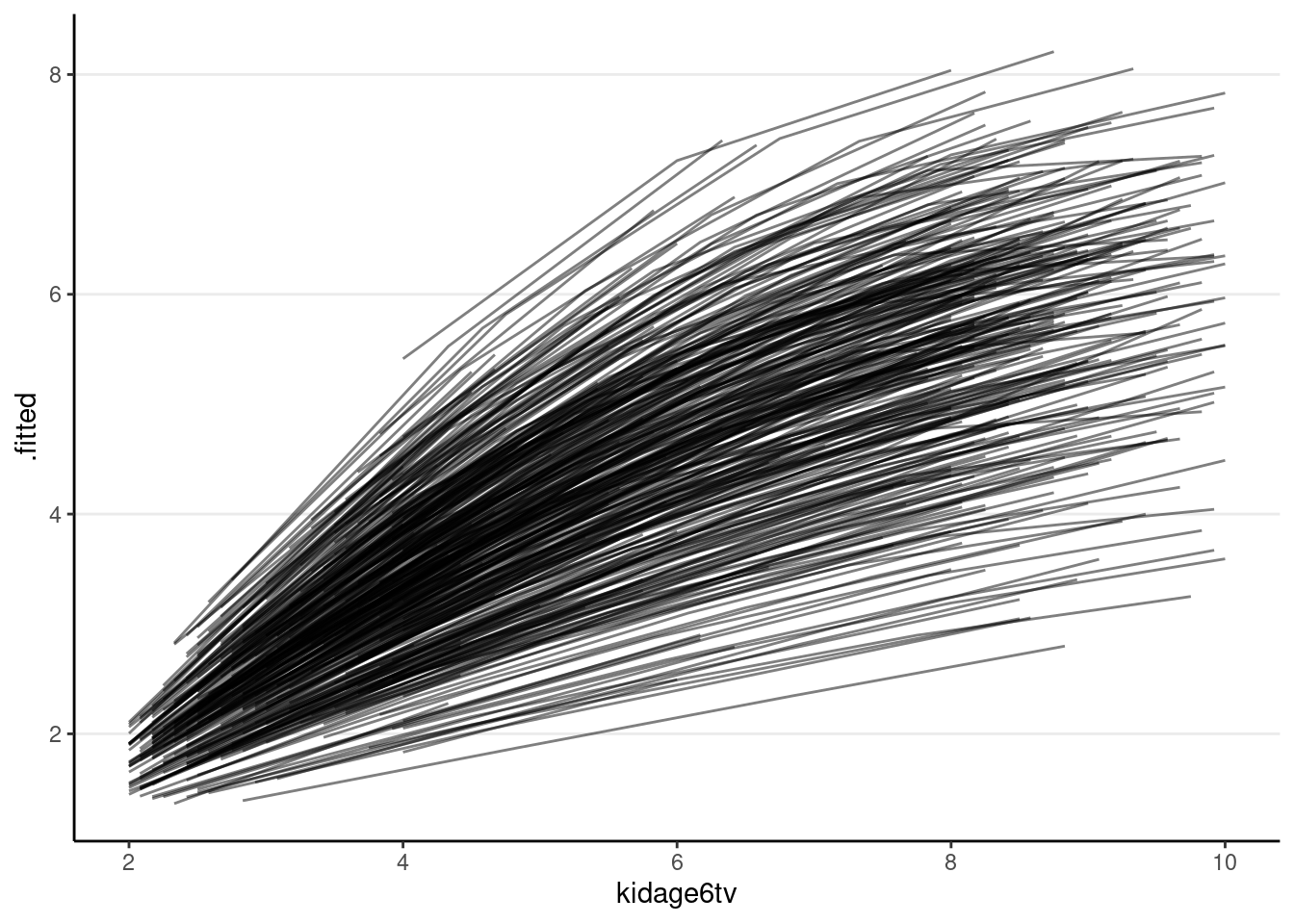
# Plot the predicted trajectories on the same panel
broom.mixed::augment(m_agesq) %>%
    ggplot(aes(x = kidage6tv, y = .fitted, group = factor(id))) +
    geom_line(alpha = 0.5)