Week 7 (R): Power

Important

There have been some updates to the R code since the videos were recorded. The major changes are:

The code now uses the packaged simr::powerCurve() function, instead of the functions I previously made, to obtain power estimates across different levels of sample sizes
For some of the examples, I started with a bigger number of clusters and cluster size, which may give more stable results for continuous predictors.

Load Packages

# To install a package, run the following ONCE (and only once on your computer)
# install.packages("simr")  
library(tidyverse)
library(lme4)
library(simr)
library(MuMIn)  # you can use `performance::r2()` as an alternative

See also an example from the vignette of the simr package: https://cran.r-project.org/web/packages/simr/vignettes/fromscratch.html

Note: In the examples of this note I used 100 simulation samples only to save time. In practice, you should use at least 1,000 to obtain a reasonable precision on the power estimation.

Binary Predictor at Level 2

$\begin{aligned} Y_{i j} & = β_{0 j} + e_{i j} \\ β_{0 j} & = γ_{00} + γ_{01} T_{j} + u_{0 j} \end{aligned}$

Preparing simulated data

First, generate the predictor matrix and the cluster ID

# Cluster ID (start with 10 clusters)
num_clus <- 10
id <- 1:num_clus
# Binary lv-2 predictor
treat <- factor(c("c", "t"))
# Level-2 data (note: `tibble` is the tidyverse version of `data.frame`)
lv2_dat <- tibble(id, treat = rep_len(treat, length.out = num_clus))
# Cluster size
clus_size <- 5
# Expand each cluster to include more rows
(sim_dat <- lv2_dat %>%
    # seq_len(n()) creates a range from 1 to number of rows
    slice(rep(seq_len(n()), each = clus_size)))

ABCDEFGHIJ0123456789

id <int>	treat <fct>
1	c
1	c
1	c
1	c
1	c
2	t
2	t
2	t
2	t
2	t

Then specify the fixed effect coefficients and the random effect variance:

gams <- c(0, 0.625)  # gamma_00, gamma_01
taus <- matrix(0.25)  # conditional ICC = 0.25 / (1 + 0.25) = 0.2
sigma <- 1  # sigma, usually fixed to be 1.0 for easier scaling

Use simr::makeLmer() to build an artificial lmer object:

sim_m1 <- makeLmer(y ~ treat + (1 | id),
                   fixef = gams, VarCorr = taus, sigma = sigma,
                   data = sim_dat)
# Check R^2
r.squaredGLMM(sim_m1)

># Warning: 'r.squaredGLMM' now calculates a revised statistic. See the help page.

>#             R2m       R2c
># [1,] 0.07383343 0.2590667

# Cohen's d
gams[2] / sqrt(taus + sigma^2)  # treatment effect / sqrt(tau_0^2 + sigma^2)

>#          [,1]
># [1,] 0.559017

Obtain simulation-based power

Now, check the power:

power_m1 <- powerSim(sim_m1,
                     # number of simulated samples; use a small number for
                     # trial run
                     nsim = 20,
                     progress = FALSE)  # suppress the progress bar
power_m1

># Power for predictor 'treat', (95% confidence interval):
>#       25.00% ( 8.66, 49.10)
># 
># Test: Likelihood ratio
># 
># Based on 20 simulations, (0 warnings, 0 errors)
># alpha = 0.05, nrow = 50
># 
># Time elapsed: 0 h 0 m 1 s

Power was obviously not sufficient as it is far from 80%, so we’ll increase it.

Increasing number of clusters

Increase to 50 clusters

(Note that I set the cache = TRUE option so that I can reuse the results next time.)

sim_m1_50J <- extend(sim_m1,
                     along = "id",  # add more levels of `id` (i.e., clusters)
                     n = 50)  # increase to 50 clusters
power_m1_50J <- powerSim(sim_m1_50J, nsim = 20, progress = FALSE)
power_m1_50J

># Power for predictor 'treat', (95% confidence interval):
>#       95.00% (75.13, 99.87)
># 
># Test: Likelihood ratio
># 
># Based on 20 simulations, (0 warnings, 0 errors)
># alpha = 0.05, nrow = 250
># 
># Time elapsed: 0 h 0 m 1 s

This looks close to 80%. Let’s try several numbers of clusters (10, 20, 30, 40, 50) with a larger nsim. You can use the simr::powerCurve() function.

# The first argument needs to be the output from running `extend`
powers_m1 <- powerCurve(
    sim_m1_50J,
    along = "id",
    breaks = c(10, 20, 30, 40, 50),
    nsim = 100,
    progress = FALSE  # suppress progress bar (for printing purpose)
)
powers_m1  # summary; check the numbers of rows are correct

># Power for predictor 'treat', (95% confidence interval),
># by largest value of id:
>#      10: 37.00% (27.56, 47.24) - 50 rows
>#      20: 51.00% (40.80, 61.14) - 100 rows
>#      30: 65.00% (54.82, 74.27) - 150 rows
>#      40: 80.00% (70.82, 87.33) - 200 rows
>#      50: 90.00% (82.38, 95.10) - 250 rows
># 
># Time elapsed: 0 h 0 m 33 s

plot(powers_m1)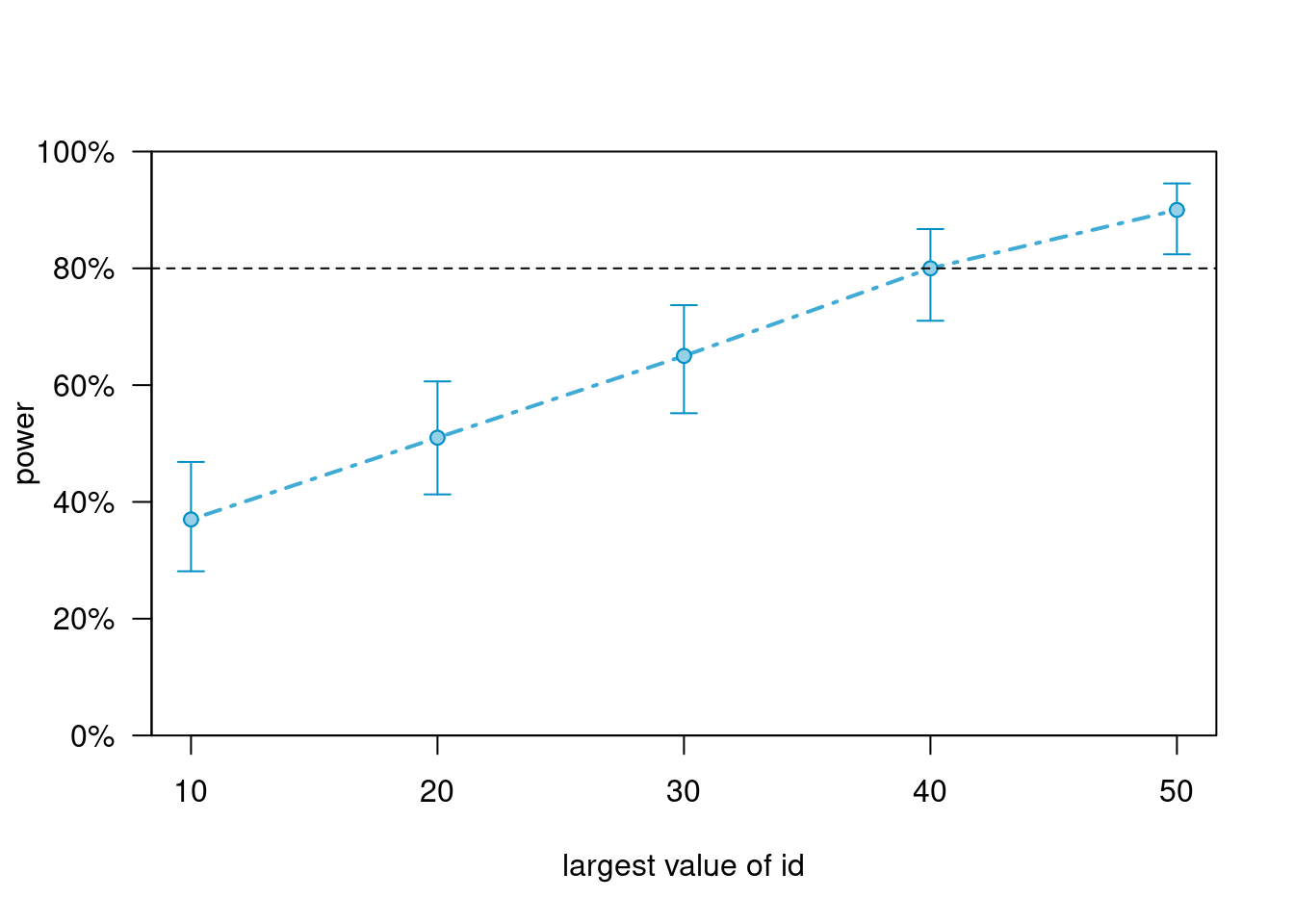

This suggests that ~ 50 clusters are needed, if each cluster contains 5 observations.

Increasing cluster size

Instead of increasing the number of cluster, one can also increase the cluster size (with $J$ = 50):

sim_m1_25n <- extend(sim_m1,
                     # need to specify the combination of id and lv-2 predictors
                     within = "id + treat",
                     n = 25)  # cluster size
power_m1_25n <- powerSim(sim_m1_25n, nsim = 100, progress = FALSE)
power_m1_25n

># Power for predictor 'treat', (95% confidence interval):
>#       52.00% (41.78, 62.10)
># 
># Test: Likelihood ratio
># 
># Based on 100 simulations, (0 warnings, 0 errors)
># alpha = 0.05, nrow = 250
># 
># Time elapsed: 0 h 0 m 8 s

Note that the power of increasing cluster size by 5 times is much smaller than that of increasing number of clusters by 5 times. Here is the power curve:

powers_m1_n <- powerCurve(
    sim_m1_25n,
    within = "id + treat",
    breaks = c(5, 10, 15, 20, 25),
    nsim = 100,
    progress = FALSE
)
powers_m1_n

># Power for predictor 'treat', (95% confidence interval),
># by number of observations within id + treat:
>#       5: 37.00% (27.56, 47.24) - 50 rows
>#      10: 44.00% (34.08, 54.28) - 100 rows
>#      15: 49.00% (38.86, 59.20) - 150 rows
>#      20: 49.00% (38.86, 59.20) - 200 rows
>#      25: 48.00% (37.90, 58.22) - 250 rows
># 
># Time elapsed: 0 h 0 m 35 s

plot(powers_m1_n)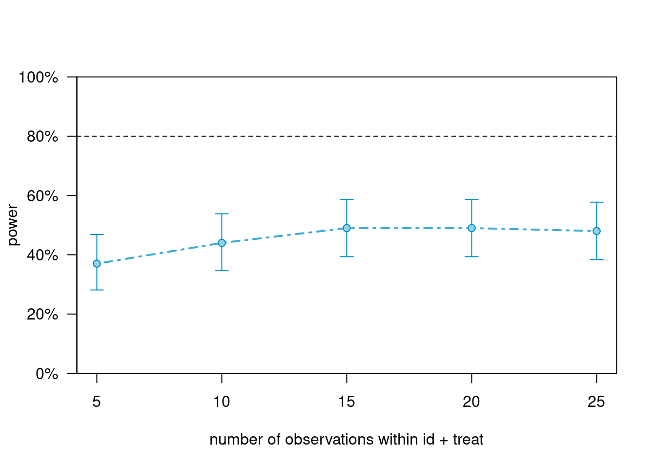

In this case, increasing the cluster size only increases the power to close to 50%. There is an upper limit in power improvement with increasing the cluster size, when the number of cluster is kept constant.

Changing effect size

Finally, we can also explore how effect size affects power

# Change gamma_01
gams <- c(0, 0.9)  # gamma_00, gamma_01
taus <- matrix(0.25)  # conditional ICC = 0.25 / (1 + 0.25) = 0.2
sigma <- 1  # sigma, usually fixed to be 1.0 for easier scaling
# Use `makeLmer()` again
sim_m1_large_es <- makeLmer(y ~ treat + (1 | id),
                            fixef = gams, VarCorr = taus, sigma = sigma,
                            data = sim_dat)
# Check R^2
r.squaredGLMM(sim_m1_large_es)

>#            R2m       R2c
># [1,] 0.1418564 0.3134851

# Cohen's d
gams[2] / sqrt(taus + sigma^2)  # treatment effect / sqrt(tau_0^2 + sigma^2)

>#           [,1]
># [1,] 0.8049845

Let’s also look at varying number of clusters

sim_m1_large_es_40J <- extend(sim_m1_large_es, along = "id", n = 40)
power_m1_large_es <- powerCurve(
    sim_m1_large_es_40J, along = "id", breaks = c(10, 20, 30, 40),
    nsim = 100, progress = FALSE
)
power_m1_large_es

># Power for predictor 'treat', (95% confidence interval),
># by largest value of id:
>#      10: 67.00% (56.88, 76.08) - 50 rows
>#      20: 86.00% (77.63, 92.13) - 100 rows
>#      30: 96.00% (90.07, 98.90) - 150 rows
>#      40: 99.00% (94.55, 99.97) - 200 rows
># 
># Time elapsed: 0 h 0 m 28 s

plot(power_m1_large_es)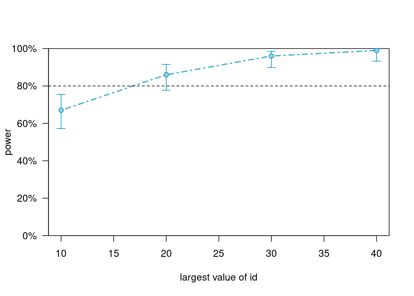

So, to summarize power for the different scenarios, if we want 80% power, we need

Treatment effect = 0.625, ~ 50 clusters
Treatment effect = 0.90, ~ 25 clusters

Continuous Predictor at Level 2

$\begin{aligned} Y_{i j} & = β_{0 j} + e_{i j} \\ β_{0 j} & = γ_{00} + γ_{01} W_{j} + u_{0 j} \end{aligned}$

Preparing Simulated Data

In the previous section, we started with a small simulated data. When we have continuous predictor(s), it is usually best to start with a larger number of clusters.

First, generate the predictor matrix and the cluster ID

# Cluster ID (use 100 clusters)
num_clus <- 100
id <- 1:num_clus
# Continuous lv-2 predictor
w <- rnorm(num_clus)
# Convert to z score so that SD = 1
w <- (w - mean(w)) / sd(w) * (num_clus - 1) / num_clus
# Level-2 data
lv2_dat <- tibble(id, w = w)
# Cluster size
clus_size <- 25
# Expand each cluster to include more rows
(sim_dat <- lv2_dat %>%
    # seq_len(n()) creates a range from 1 to number of rows
    slice(rep(seq_len(n()), each = clus_size)))

ABCDEFGHIJ0123456789

id <int>	w <dbl>
1	-0.093576722
1	-0.093576722
1	-0.093576722
1	-0.093576722
1	-0.093576722
1	-0.093576722
1	-0.093576722
1	-0.093576722
1	-0.093576722
1	-0.093576722

Then specify the fixed effect coefficients and the random effect variance:

gams <- c(1, 0.3)  # gamma_00, gamma_01
taus <- matrix(0.5)  # conditional ICC = 0.5 / (1 + 0.5) = 0.33
sigma <- 1  # sigma, usually fixed to be 1.0 for easier scaling

Use simr::makeLmer() to build an artificial lmer object:

sim_m2 <- makeLmer(y ~ w + (1 | id),
                   fixef = gams, VarCorr = taus, sigma = sigma,
                   data = sim_dat)
# Check R^2
r.squaredGLMM(sim_m2)

>#             R2m       R2c
># [1,] 0.05503588 0.3700239

Obtain simulation-based power

Use various numbers of clusters

powers_m2 <- powerCurve(
    sim_m2, along = "id", breaks = c(10, 20, 50, 100),
    nsim = 100, progress = FALSE
)
powers_m2

># Power for predictor 'w', (95% confidence interval),
># by largest value of id:
>#      10: 26.00% (17.74, 35.73) - 250 rows
>#      20: 37.00% (27.56, 47.24) - 500 rows
>#      50: 74.00% (64.27, 82.26) - 1250 rows
>#     100: 99.00% (94.55, 99.97) - 2500 rows
># 
># Time elapsed: 0 h 4 m 54 s

plot(powers_m2)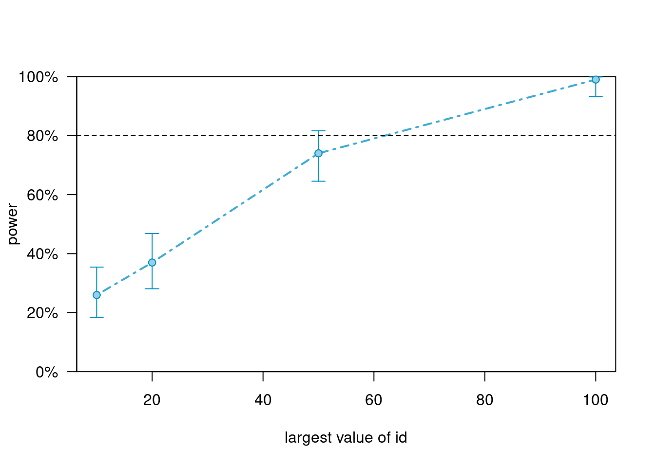

Use various cluster sizes (negligible change in power)

powers_m2_n <- powerCurve(
    sim_m2, within = "id + w", breaks = c(5, 10, 25, 50),
    nsim = 100, progress = FALSE
)
powers_m2_n

># Power for predictor 'w', (95% confidence interval),
># by number of observations within id + w:
>#       5: 94.00% (87.40, 97.77) - 500 rows
>#      10: 98.00% (92.96, 99.76) - 1000 rows
>#      25: 99.00% (94.55, 99.97) - 2500 rows
>#      NA: 99.00% (94.55, 99.97) - 2500 rows
># 
># Time elapsed: 0 h 6 m 19 s

plot(powers_m2_n)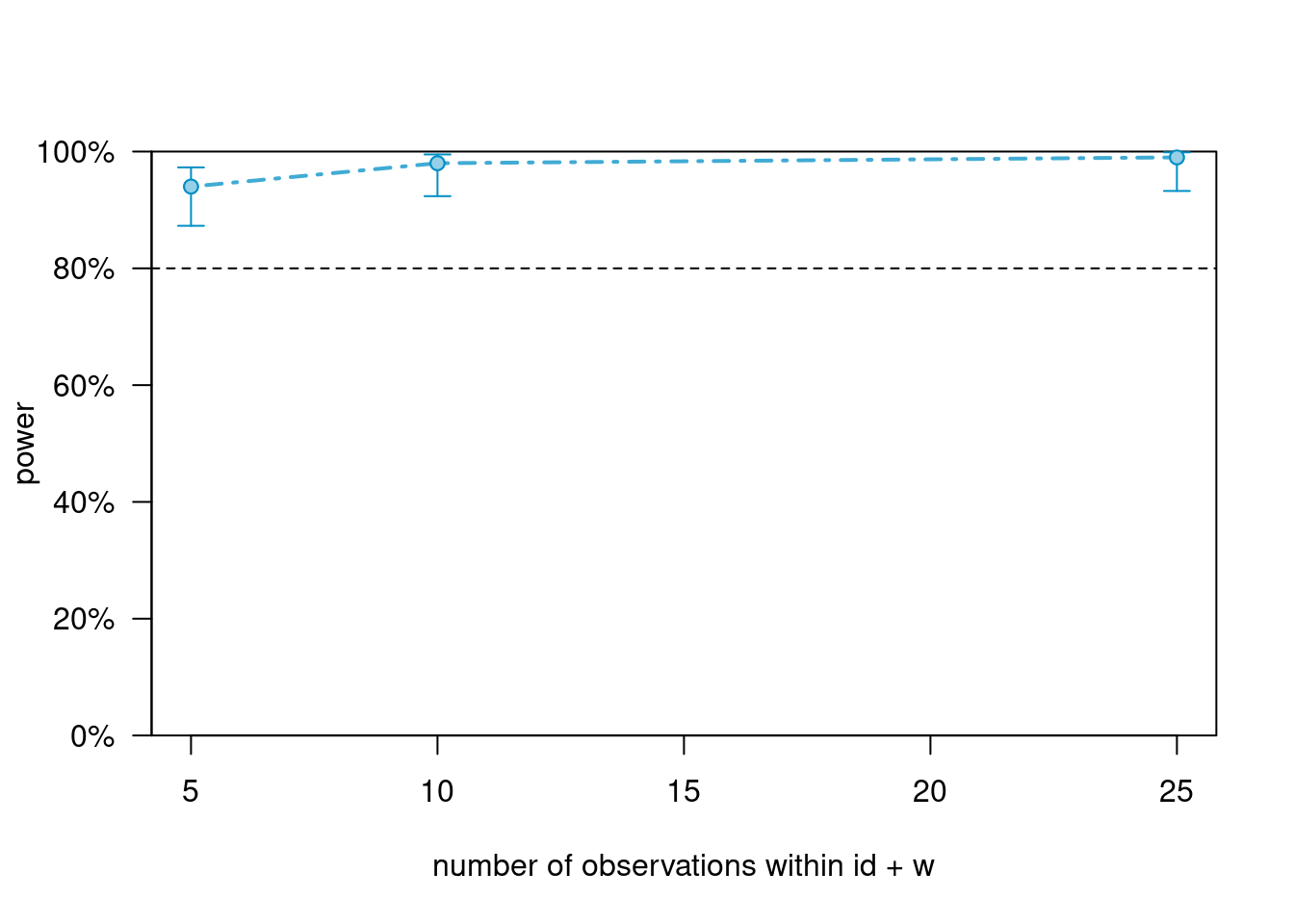

Binary Predictor at Level 2 With a Continuous Level-1 Covariate (and Random Slope)

Cluster-mean centering needs to be considerd

$\begin{aligned} Y_{i j} & = β_{0 j} + β_{1 j} X {_cmc}_{i j} + e_{i j} \\ β_{0 j} & = γ_{00} + γ_{01} W_{j} + γ_{02} X {_cm}_{j} + u_{0 j} \\ β_{1 j} & = γ_{10} + γ_{11} W_{j} + u_{1 j} \end{aligned}$

We consider a covariate with ICC = .2

Preparing Simulated Data

First, generate the simulated data. I use a large $J$ and a moderate $n$ here.

# Step 1: Lv-2 data (basically the same as before)
# Cluster ID (start with 10 clusters)
num_clus <- 100
id <- 1:num_clus
# Binary lv-2 predictor
treat <- factor(c("c", "t"))
# Cluster means of X, with ICC(X) = 0.2
x_cm <- rnorm(num_clus, mean = 0, sd = sqrt(0.2))
# Force SD = sqrt(0.2)
x_cm <- (x_cm - mean(x_cm)) / sd(x_cm) * sqrt(0.2) * (num_clus - 1) / num_clus
# Level-2 data
lv2_dat <- tibble(id, treat = rep_len(treat, length.out = num_clus), x_cm)
# Expand each cluster to include more rows
clus_size <- 40  # Cluster size
sim_dat <- lv2_dat %>%
    slice(rep(seq_len(n()), each = clus_size))

# Step 2: Add level-1 covariate
# Within-cluster component of X, with sigma^2(X) = 0.8
num_obs <- num_clus * clus_size
x_cmc <- rnorm(num_obs, mean = 0, sd = 1)
x_cmc <- x_cmc - ave(x_cmc, lv2_dat$id, FUN = mean)
# Force SD = sqrt(0.8)
x_cmc <- x_cmc / sd(x_cmc) * sqrt(0.8) * (num_obs - 1) / num_obs
# Add `x_cmc` to `sim_dat`
sim_dat$x_cmc <- x_cmc

Then specify the fixed effect coefficients and the random effect variance:

# gamma_00, gamma_01, gamma_02, gamma_10, gamma_11
gams <- c(0, 0.3, 0.2, 0.1, 0.2)
taus <- matrix(c(0.25, 0,
                 0, 0.10), nrow = 2)  # tau^2_0 = 0.25, tau^2_1 = 0.1
sigma <- sqrt(.96)  # sigma

Use simr::makeLmer() to build an artificial lmer object:

sim_m4 <- makeLmer(y ~ treat + x_cm + x_cmc + treat:x_cmc + (x_cmc | id),
                   fixef = gams, VarCorr = taus, sigma = sigma,
                   data = sim_dat)
# Check R^2
r.squaredGLMM(sim_m4)

>#            R2m      R2c
># [1,] 0.0528709 0.295127

# Compare to a model without the cross-level interaction
sim_m4null <- makeLmer(y ~ treat + x_cm + x_cmc + (x_cmc | id),
                       fixef = gams[1:4], VarCorr = taus, sigma = sigma,
                       data = sim_dat)
# Check R^2
r.squaredGLMM(sim_m4null)

>#             R2m       R2c
># [1,] 0.02919444 0.2775064

# So the cross-level interaction corresponds to an R^2 change of about 2.5%

Obtain simulation-based power

Use various numbers of clusters

(Note: by default the first term in the fixed effect [other than the intercept] will be tested. We’ll specify the interaction instead.)

powers_m4 <- powerCurve(
    sim_m4, along = "id", breaks = c(10, 20, 50, 100),
    # `method = "anova"` means power for LRT
    test = fixed("treat:x_cmc", method = "anova"),
    nsim = 100, progress = FALSE
)
powers_m4

># Power for predictor 'treat:x_cmc', (95% confidence interval),
># by largest value of id:
>#      10: 11.00% ( 5.62, 18.83) - 400 rows
>#      20: 20.00% (12.67, 29.18) - 800 rows
>#      50: 50.00% (39.83, 60.17) - 2000 rows
>#     100: 80.00% (70.82, 87.33) - 4000 rows
># 
># Time elapsed: 0 h 1 m 11 s

plot(powers_m4)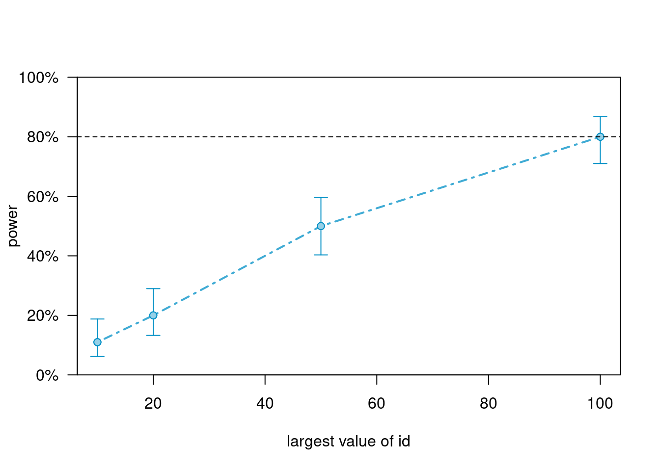

Use various cluster sizes (results not shown)

# Increase to n = 200
sim_m4_200n <- extend(sim_m4, within = "id + treat + x_cm", n = 200)
# Decrease to J = 50
sim_m4_200n <- extend(sim_m4_200n, along = "id", n = 50)
powers_m4_n <- powerCurve(
    sim_m4_200n, within = "id + treat + x_cm", breaks = c(40, 80, 200),
    # `method = "anova"` means power for LRT
    test = fixed("treat:x_cmc", method = "anova"),
    nsim = 100, progress = FALSE
)
powers_m4_n
plot(powers_m4_n)

Bonus: Growth Modeling

With a binary person-level predictor

$\begin{aligned} Y_{t i} & = β_{0 j} + β_{1 i} {time}_{t i} + e_{t i} \\ β_{0 i} & = γ_{00} + γ_{01} W_{i} + u_{0 i} \\ β_{1 i} & = γ_{10} + γ_{11} W_{i} + u_{1 i} \end{aligned}$

Preparing Simulated Data

First, generate the predictor matrix and the cluster ID

# Person ID (start with 50 clusters)
num_clus <- 50
id <- 1:num_clus
# Binary lv-2 predictor
treat <- factor(c("c", "t"))
# Level-2 data
lv2_dat <- tibble(id, treat = rep_len(treat, length.out = num_clus))
# Expand each cluster to include more rows
clus_size <- 4  # Number of time points
# Within-cluster component of X, with sigma^2(X) = 0.8
time <- 1:clus_size
# Expand each cluster to include more rows
(sim_dat <- expand_grid(lv2_dat, time))

ABCDEFGHIJ0123456789

id <int>	treat <fct>	time <int>
1	c	1
1	c	2
1	c	3
1	c	4
2	t	1
2	t	2
2	t	3
2	t	4
3	c	1
3	c	2

Then specify the fixed effect coefficients and the random effect variance:

# gamma_00, gamma_01, gamma_10, gamma_11
gams <- c(1, 0, -0.2, 0.3)
taus <- matrix(c(0.5, 0,
                 0, 0.10), nrow = 2)  # tau^2_0 = 0.5, tau^2_1 = 0.1
sigma <- sqrt(1)  # sigma

Use simr::makeLmer() to build an artificial lmer object:

# I use `I(time - 1)` so that the intercept is for the first time point
sim_m5 <- makeLmer(
    y ~ treat + I(time - 1) + treat:I(time - 1) + (I(time - 1) | id),
    fixef = gams, VarCorr = taus, sigma = sigma,
    data = sim_dat
)
# Check R^2
r.squaredGLMM(sim_m5)

>#             R2m       R2c
># [1,] 0.04258501 0.4824784

# Compare to a model without the binary treatment predictor
sim_m5null <- makeLmer(y ~ I(time - 1) + (I(time - 1) | id),
                       fixef = gams[c(1, 3)], VarCorr = taus, sigma = sigma,
                       data = sim_dat)
# Check R^2
r.squaredGLMM(sim_m5null)

>#             R2m       R2c
># [1,] 0.02644453 0.4737538

# So treat and its interaction corresponds to an R^2 change of about 2%

Obtain simulation-based power

Use various numbers of clusters. The default is to test the first fixed effect (i.e., treat, group difference at the initial time point) using a likelihood ratio test. The true value of this coefficient, so the estimated power is actually Type I error in this case.

# Increase to 100 participants
sim_m5_100J <- extend(sim_m5, along = "id", n = 100)
powers_m5 <- powerCurve(
    sim_m5_100J, along = "id", breaks = c(10, 20, 50, 100),
    nsim = 100, progress = FALSE
)
powers_m5

># Power for predictor 'treat', (95% confidence interval),
># by largest value of id:
>#      10:  3.00% ( 0.62,  8.52) - 40 rows
>#      20:  5.00% ( 1.64, 11.28) - 80 rows
>#      50:  4.00% ( 1.10,  9.93) - 200 rows
>#     100:  6.00% ( 2.23, 12.60) - 400 rows
># 
># Time elapsed: 0 h 0 m 39 s

plot(powers_m5)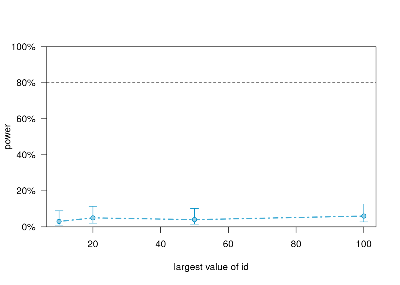

Now test the slope difference (i.e., treat:time interaction)

powers_m5_int <- powerCurve(
    sim_m5_100J, along = "id", breaks = c(10, 20, 50, 100),
    test = fixed("treat:I(time - 1)", method = "anova"),
    nsim = 100, progress = FALSE
)
plot(powers_m5_int)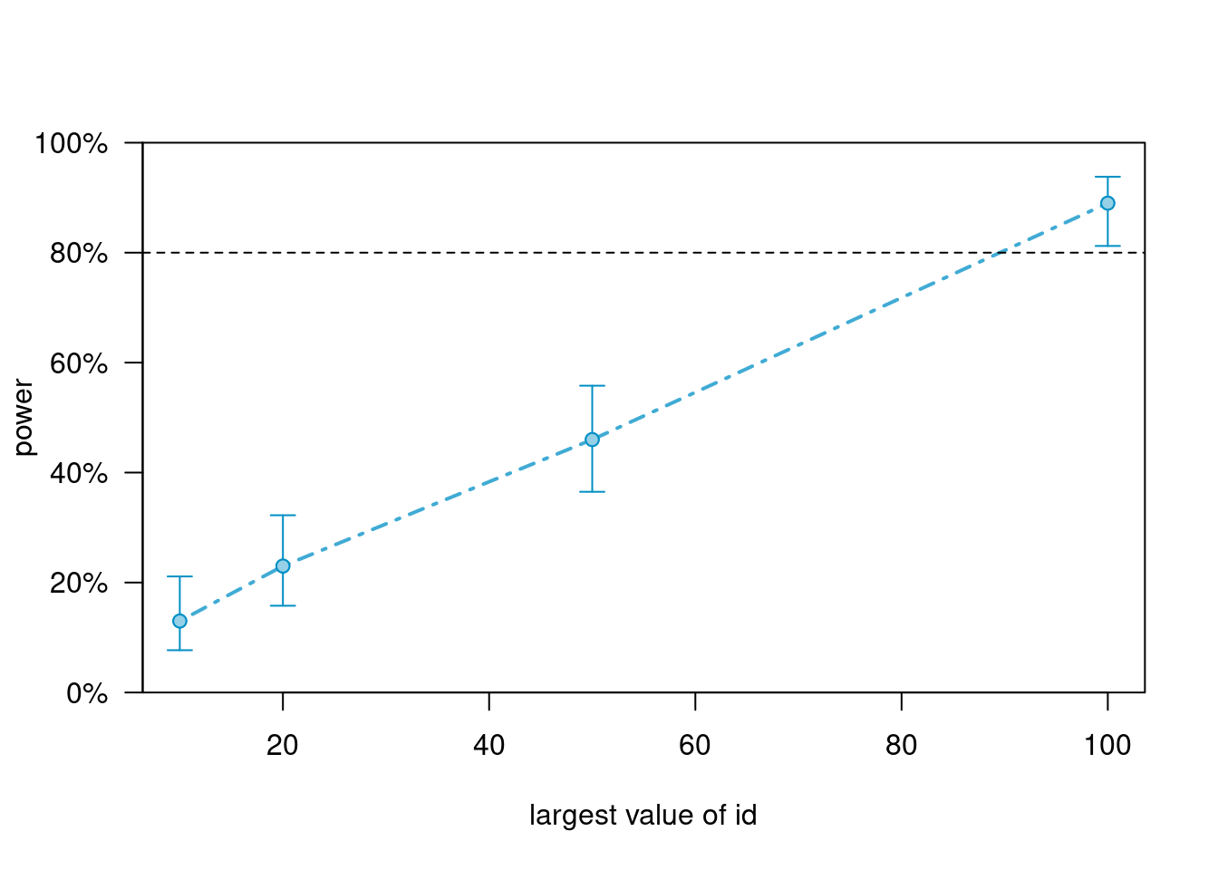

Use more time points

# Increase to 8 time points
sim_m5_50n <- extend(sim_m5, along = "time", values = 1:8)
powers_m5_n <- powerCurve(
    sim_m5_50n, along = "time", breaks = c(4, 6, 8),
    nsim = 100, progress = FALSE,
    test = fixed("treat:I(time - 1)", method = "anova")
)
powers_m5_n

># Power for predictor 'treat:I(time - 1)', (95% confidence interval),
># by largest value of time:
>#       4: 49.00% (38.86, 59.20) - 200 rows
>#       6: 82.00% (73.05, 88.97) - 300 rows
>#       8: 85.00% (76.47, 91.35) - 400 rows
># 
># Time elapsed: 0 h 0 m 25 s

plot(powers_m5_n)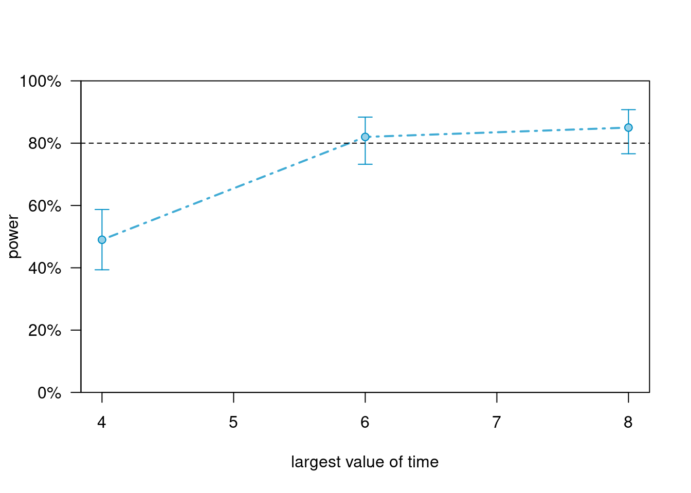

Increasing number of time points helps a little bit for testing the slope difference.