Week 4 (R): Lv-1 Predictors

Load Packages and Import Data

# To install a package, run the following ONCE (and only once on your computer)
# install.packages("psych")  
library(here)  # makes reading data more consistent
library(tidyverse)  # for data manipulation and plotting
library(haven)  # for importing SPSS/SAS/Stata data
library(lme4)  # for multilevel analysis
library(sjPlot)  # for plotting effects
library(MuMIn)  # for computing r-squared
library(broom.mixed)  # for augmenting results
library(modelsummary)  # for making tables
library(interactions)  # for plotting interactions

Import Data

# Read in the data (pay attention to the directory)
hsball <- read_sav(here("data_files", "hsball.sav"))

Between-Within Decomposition

Cluster-mean centering

To separate the effects of a lv-1 predictor into different levels, one needs to first center the predictor on the cluster means:

hsball <- hsball %>%
    group_by(id) %>%   # operate within schools
    mutate(ses_cm = mean(ses),   # create cluster means (the same as `meanses`)
           ses_cmc = ses - ses_cm) %>%   # cluster-mean centered
    ungroup()  # exit the "editing within groups" mode
# The meanses variable already exists in the original data, but it's slightly
# different from computing it by hand
hsball %>%
    select(id, ses, meanses, ses_cm, ses_cmc)

ABCDEFGHIJ0123456789

id <chr>	ses <dbl>	meanses <dbl>	ses_cm <dbl>	ses_cmc <dbl>
1224	-1.528	-0.428	-0.434382979	-1.093617e+00
1224	-0.588	-0.428	-0.434382979	-1.536170e-01
1224	-0.528	-0.428	-0.434382979	-9.361702e-02
1224	-0.668	-0.428	-0.434382979	-2.336170e-01
1224	-0.158	-0.428	-0.434382979	2.763830e-01
1224	0.022	-0.428	-0.434382979	4.563830e-01
1224	-0.618	-0.428	-0.434382979	-1.836170e-01
1224	-0.998	-0.428	-0.434382979	-5.636170e-01
1224	-0.888	-0.428	-0.434382979	-4.536170e-01
1224	-0.458	-0.428	-0.434382979	-2.361702e-02

Model Equation

Lv-1:

${mathach}_{i j} = β_{0 j} + β_{1 j} {ses_cmc}_{i j} + e_{i j}$

Lv-2:

$\begin{aligned} β_{0 j} & = γ_{00} + γ_{01} {meanses}_{j} + u_{0 j} \\ β_{1 j} & = γ_{10} \end{aligned}$ where

$γ_{10}$ = regression coefficient of student-level ses representing the expected difference in student achievement between two students in the same school with one unit difference in ses,
$γ_{01}$ = between-school effect, which is the expected difference in mean achievement between two schools with one unit difference in meanses.

Running in R

We can specify the model as:

m_bw <- lmer(mathach ~ meanses + ses_cmc + (1 | id), data = hsball)

As an alternative to creating the cluster means and centered variables in the data, you can directly create in the formula:

m_bw2 <- lmer(mathach ~ I(ave(ses, id)) + I(ses - ave(ses, id)) + (1 | id),
              data = hsball)

You can summarize the results using

summary(m_bw)

># Linear mixed model fit by REML ['lmerMod']
># Formula: mathach ~ meanses + ses_cmc + (1 | id)
>#    Data: hsball
># 
># REML criterion at convergence: 46568.6
># 
># Scaled residuals: 
>#     Min      1Q  Median      3Q     Max 
># -3.1666 -0.7253  0.0174  0.7557  2.9453 
># 
># Random effects:
>#  Groups   Name        Variance Std.Dev.
>#  id       (Intercept)  2.692   1.641   
>#  Residual             37.019   6.084   
># Number of obs: 7185, groups:  id, 160
># 
># Fixed effects:
>#             Estimate Std. Error t value
># (Intercept)  12.6481     0.1494   84.68
># meanses       5.8662     0.3617   16.22
># ses_cmc       2.1912     0.1087   20.16
># 
># Correlation of Fixed Effects:
>#         (Intr) meanss
># meanses -0.004       
># ses_cmc  0.000  0.000

Contextual Effect

With a level-1 predictor like ses, which has both student-level and school-level variance, we can include both the level-1 and the school mean variables as predictors. When the level-1 predictor is present, the coefficient for the group means variable becomes the contextual effect.

Model Equation

Lv-1:

${mathach}_{i j} = β_{0 j} + β_{1 j} {ses}_{i j} + e_{i j}$

Lv-2:

$\begin{aligned} β_{0 j} & = γ_{00} + γ_{01} {meanses}_{j} + u_{0 j} \\ β_{1 j} & = γ_{10} \end{aligned}$ where

$γ_{10}$ = regression coefficient of student-level ses representing the expected difference in student achievement between two students in the same school with one unit difference in ses,
$γ_{01}$ = contextual effect, which is the expected difference in student achievement between two students with the same ses but from two schools with one unit difference in meanses.

Running in R

We can specify the model as:

contextual <- lmer(mathach ~ meanses + ses + (1 | id), data = hsball)

You can summarize the results using

summary(contextual)

># Linear mixed model fit by REML ['lmerMod']
># Formula: mathach ~ meanses + ses + (1 | id)
>#    Data: hsball
># 
># REML criterion at convergence: 46568.6
># 
># Scaled residuals: 
>#     Min      1Q  Median      3Q     Max 
># -3.1666 -0.7253  0.0174  0.7557  2.9453 
># 
># Random effects:
>#  Groups   Name        Variance Std.Dev.
>#  id       (Intercept)  2.692   1.641   
>#  Residual             37.019   6.084   
># Number of obs: 7185, groups:  id, 160
># 
># Fixed effects:
>#             Estimate Std. Error t value
># (Intercept)  12.6613     0.1494  84.763
># meanses       3.6750     0.3777   9.731
># ses           2.1912     0.1087  20.164
># 
># Correlation of Fixed Effects:
>#         (Intr) meanss
># meanses -0.005       
># ses      0.004 -0.288

If you compare the REML criterion at convergence number, you can see this is the same as the between-within model. The estimated contextual effect is the coefficient of meanses minus the coefficient of ses_cmc, which is the same as what you will get in the contextual effect model.

Random-Coefficients Model

Explore Variations in Slopes

hsball %>%
    # randomly sample 16 schools
    filter(id %in% sample(unique(id), 16)) %>%
    # ses on x-axis and mathach on y-axis
    ggplot(aes(x = ses, y = mathach)) +
    # add points (half the original size)
    geom_point(size = 0.5) +
    # add a linear smoother
    geom_smooth(method = "lm") +
    # present data of different ids in different panels
    facet_wrap(~id)

># `geom_smooth()` using formula = 'y ~ x'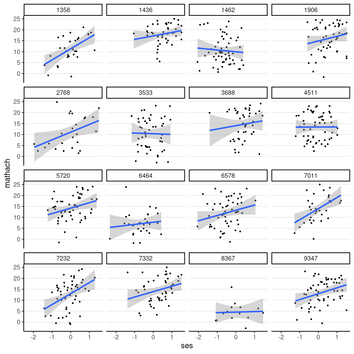

Model Equation

Lv-1:

${mathach}_{i j} = β_{0 j} + β_{1 j} {ses_cmc}_{i j} + e_{i j}$

Lv-2:

$\begin{aligned} β_{0 j} & = γ_{00} + γ_{01} {meanses}_{j} + u_{0 j} \\ β_{1 j} & = γ_{10} + u_{1 j} \end{aligned}$ The additional term is $u_{1 j}$ , which represents the deviation of the slope of school $j$ from the average slope (i.e., $γ_{10}$ ).

Running in R

We have to put ses in the random part:

ran_slp <- lmer(mathach ~ meanses + ses_cmc + (ses_cmc | id), data = hsball)

You can summarize the results using

summary(ran_slp)

># Linear mixed model fit by REML ['lmerMod']
># Formula: mathach ~ meanses + ses_cmc + (ses_cmc | id)
>#    Data: hsball
># 
># REML criterion at convergence: 46557.7
># 
># Scaled residuals: 
>#     Min      1Q  Median      3Q     Max 
># -3.1768 -0.7269  0.0160  0.7560  2.9406 
># 
># Random effects:
>#  Groups   Name        Variance Std.Dev. Corr 
>#  id       (Intercept)  2.6931  1.6411        
>#           ses_cmc      0.6858  0.8281   -0.19
>#  Residual             36.7132  6.0591        
># Number of obs: 7185, groups:  id, 160
># 
># Fixed effects:
>#             Estimate Std. Error t value
># (Intercept)  12.6454     0.1492   84.74
># meanses       5.8963     0.3600   16.38
># ses_cmc       2.1913     0.1280   17.11
># 
># Correlation of Fixed Effects:
>#         (Intr) meanss
># meanses -0.004       
># ses_cmc -0.088  0.004

Showing the random intercepts and slopes

head(coef(ran_slp)$id)  # `head()` shows only the first six schools

ABCDEFGHIJ0123456789

	(Intercept) <dbl>	meanses <dbl>	ses_cmc <dbl>
1224	12.32411	5.896293	2.292981
1288	12.69256	5.896293	2.359732
1296	10.70293	5.896293	2.040818
1308	12.94395	5.896293	2.013578
1317	11.46711	5.896293	2.092983
1358	11.64868	5.896293	2.800057

Plotting Random Slopes

# The `augment` function adds predicted values to the data
augment(ran_slp, data = hsball) %>%
    ggplot(aes(x = ses, y = .fitted, color = factor(id))) +
    geom_smooth(method = "lm", se = FALSE, size = 0.5) +
    labs(y = "Predicted mathach") +
    guides(color = "none")

># Warning: Using `size` aesthetic for lines was deprecated in ggplot2 3.4.0.
># ℹ Please use `linewidth` instead.

># `geom_smooth()` using formula = 'y ~ x'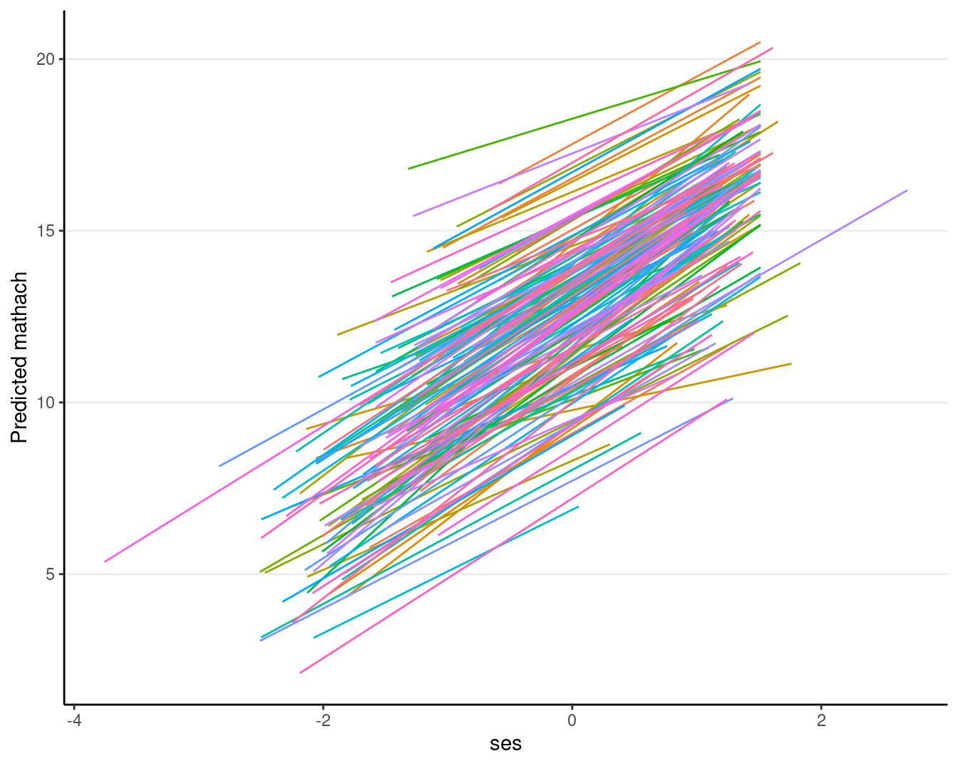

Or using sjPlot::plot_model() (with ses_cmc, not ses, on the x-axis)

plot_model(ran_slp, type = "pred", pred.type = "re", terms = c("ses_cmc", "id"),
           # suppress confidence band
           ci.lvl = NA, show.legend = FALSE, colors = "gs")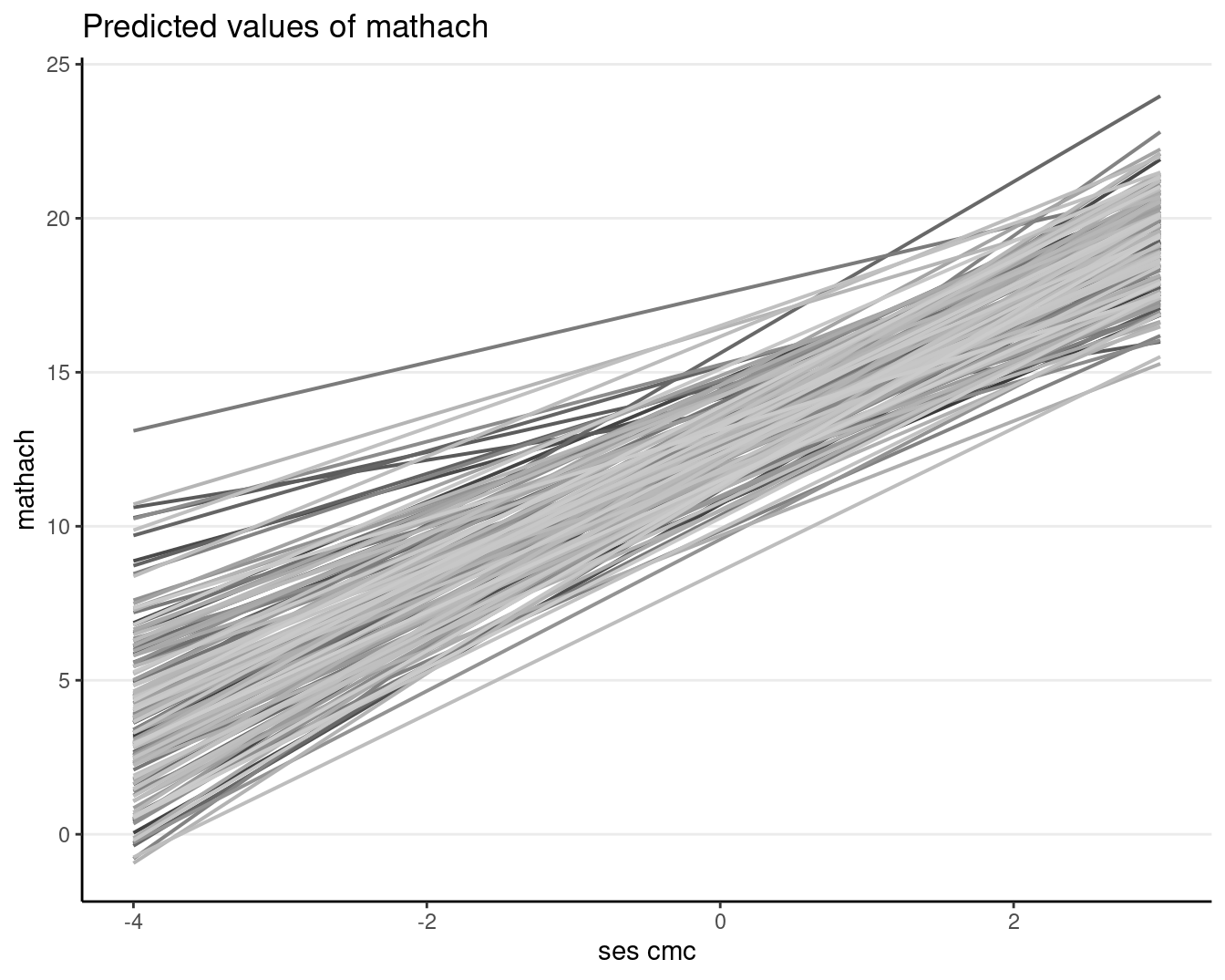

Including the effect of `meanses`

# augmented data (adding EB estimates)
augment(ran_slp, data = hsball) %>%
    ggplot(aes(x = ses, y = mathach, color = factor(id))) +
    # Add points
    geom_point(size = 0.2, alpha = 0.2) +
    # Add within-cluster lines
    geom_smooth(aes(y = .fitted),
                method = "lm", se = FALSE, size = 0.5) +
    # Add group means with `stat_summary`
    stat_summary(aes(x = meanses, y = .fitted,
                     fill = factor(id)),
                 fun = mean,
                 geom = "point",
                 color = "red",  # add border
                 shape = 24, # use triangles
                 size = 2.5) +
    # Add between coefficient
    geom_smooth(aes(x = meanses, y = .fitted),
                method = "lm", se = FALSE,
                color = "black") +
    labs(y = "Math Achievement") +
    # Suppress legend as there are too many schools
    guides(color = "none", fill = "none")

># `geom_smooth()` using formula = 'y ~ x'
># `geom_smooth()` using formula = 'y ~ x'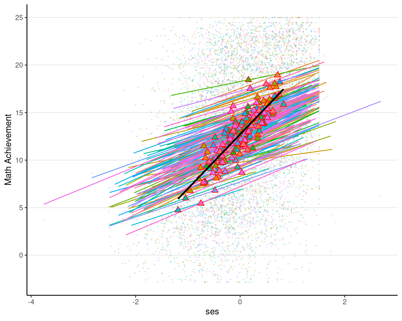

Or on separate graphs:

# Create a common base graph
pbase <- augment(ran_slp, data = hsball) %>%
    ggplot(aes(x = ses, y = mathach, color = factor(id))) +
    # Add points
    geom_point(size = 0.2, alpha = 0.2) +
    labs(y = "Math Achievement") +
    # Suppress legend
    guides(color = "none")
# Lv-1 effect
p1 <- pbase +
    # Add within-cluster lines
    geom_smooth(aes(y = .fitted),
                method = "lm", se = FALSE, size = 0.5)
# Lv-2 effect
p2 <- pbase +
    # Add group means
    stat_summary(aes(x = meanses, y = .fitted),
                 fun = mean,
                 geom = "point",
                 shape = 17, # use triangles
                 size = 2.5) +
    # Add between coefficient
    geom_smooth(aes(x = meanses, y = .fitted),
                method = "lm", se = FALSE,
                color = "black")
# Put the two graphs together (need the gridExtra package)
gridExtra::grid.arrange(p1, p2, ncol = 2)  # in two columns

># `geom_smooth()` using formula = 'y ~ x'
># `geom_smooth()` using formula = 'y ~ x'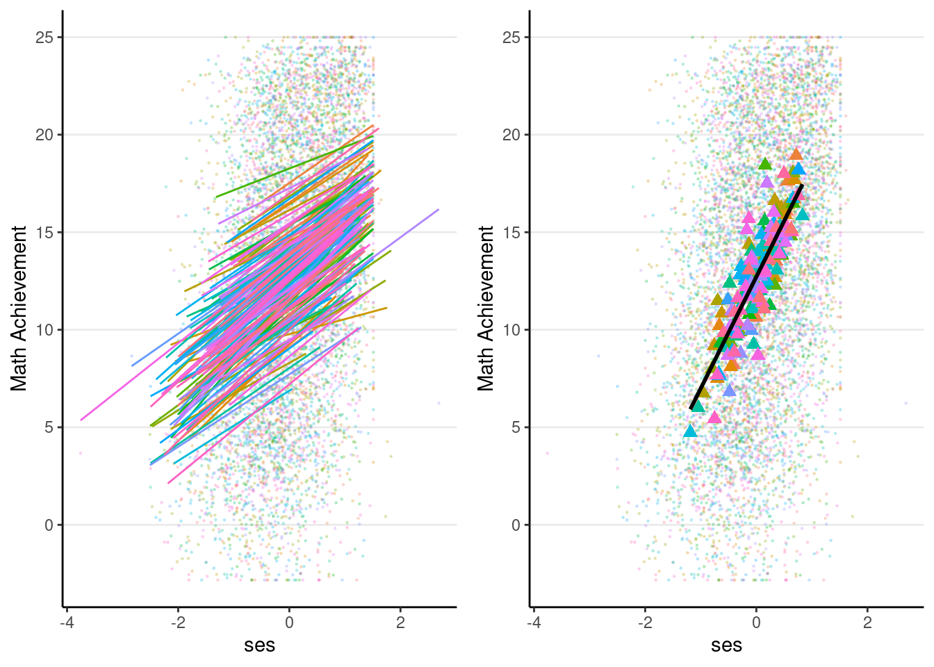

Effect Size

As discussed in the previous week, we can obtain the effect size ( $R^{2}$ ) for the model:

(r2_ran_slp <- r.squaredGLMM(ran_slp))

># Warning: 'r.squaredGLMM' now calculates a revised statistic. See the help page.

>#            R2m       R2c
># [1,] 0.1684161 0.2310862

Analyzing Cross-Level Interactions

sector is added to the level-2 intercept and slope equations.

Model Equation

Lv-1:

${mathach}_{i j} = β_{0 j} + β_{1 j} {ses_cmc}_{i j} + e_{i j}$

Lv-2:

$\begin{aligned} β_{0 j} & = γ_{00} + γ_{01} {meanses}_{j} + γ_{02} {sector}_{j} + u_{0 j} \\ β_{1 j} & = γ_{10} + γ_{11} {sector}_{j} + u_{1 j} \end{aligned}$ where - $γ_{02}$ = regression coefficient of school-level sector variable representing the expected difference in achievement between two students with the same SES level and from two schools with the same school-level SES, but one is a catholic school and the other a private school. - $γ_{11}$ = cross-level interaction coefficient of the expected slope difference between a catholic and a private school with the same school-level SES.

Running in R

We have to put the sector * ses interaction to the fixed part:

# The first step is optional, but let's recode sector into a factor variable
hsball <- hsball %>%
    mutate(sector = factor(sector, levels = c(0, 1),
                           labels = c("Public", "Catholic")))
crlv_int <- lmer(mathach ~ meanses + sector * ses_cmc + (ses_cmc | id),
                 data = hsball)

You can summarize the results using

summary(crlv_int)

># Linear mixed model fit by REML ['lmerMod']
># Formula: mathach ~ meanses + sector * ses_cmc + (ses_cmc | id)
>#    Data: hsball
># 
># REML criterion at convergence: 46514.5
># 
># Scaled residuals: 
>#      Min       1Q   Median       3Q      Max 
># -3.11560 -0.72905  0.01592  0.75280  3.01543 
># 
># Random effects:
>#  Groups   Name        Variance Std.Dev. Corr
>#  id       (Intercept)  2.3807  1.5430       
>#           ses_cmc      0.2716  0.5212   0.24
>#  Residual             36.7077  6.0587       
># Number of obs: 7185, groups:  id, 160
># 
># Fixed effects:
>#                        Estimate Std. Error t value
># (Intercept)             12.0846     0.1987   60.81
># meanses                  5.2450     0.3682   14.24
># sectorCatholic           1.2523     0.3062    4.09
># ses_cmc                  2.7877     0.1559   17.89
># sectorCatholic:ses_cmc  -1.3478     0.2348   -5.74
># 
># Correlation of Fixed Effects:
>#             (Intr) meanss sctrCt ss_cmc
># meanses      0.245                     
># sectorCthlc -0.697 -0.355              
># ses_cmc      0.071 -0.002 -0.046       
># sctrCthlc:_ -0.048 -0.001  0.071 -0.664

Effect Size

By comparing the $R^{2}$ of this model (with interaction) and the previous model (without the interaction), we can obtain the proportion of variance accounted for by the cross-level interaction:

(r2_crlv_int <- r.squaredGLMM(crlv_int))

>#            R2m       R2c
># [1,] 0.1759122 0.2284431

# Change
r2_crlv_int - r2_ran_slp

>#              R2m          R2c
># [1,] 0.007496143 -0.002643047

Therefore, the cross-level interaction between sector and SES accounted for an effect size of $Δ R^{2}$ = 0.7%. This is usually considered a small effect size (i.e., < 1%), but interpreting the magnitude of an effect size needs to take into account the area of research, the importance of the outcome, and the effect sizes when using other predictors to predict the same outcome.

Simple Slopes

With a cross-level interaction, the slope between ses_cmc and mathach depends on a moderator, sector. To find out what the model suggests to be the slope at a particular level of sector, which is also called a simple slope in the literature, you just need to look at the equation for $β_{1 j}$ , which shows that the predicted slope is ${\hat{β}}_{1} = {\hat{γ}}_{10} + {\hat{γ}}_{11} sector .$ So when sector = 0 (public school), the simple slope is ${\hat{β}}_{1} = {\hat{γ}}_{10} + {\hat{γ}}_{11} (0),$ or 2.7877417. When sector = 1 (private school), the simple slope is ${\hat{β}}_{1} = {\hat{γ}}_{10} + {\hat{γ}}_{11} (1),$ or 2.7877417 + (-1.3477638)(1) = 1.4399779.

Plotting the Interactions

crlv_int %>%
    augment(data = hsball) %>%
    ggplot(aes(
      x = ses, y = .fitted, group = factor(id),
      color = factor(sector)  # use `sector` for coloring lines
    )) +
    geom_smooth(method = "lm", se = FALSE, size = 0.5) +
    labs(y = "Predicted mathach", color = "sector")

># `geom_smooth()` using formula = 'y ~ x'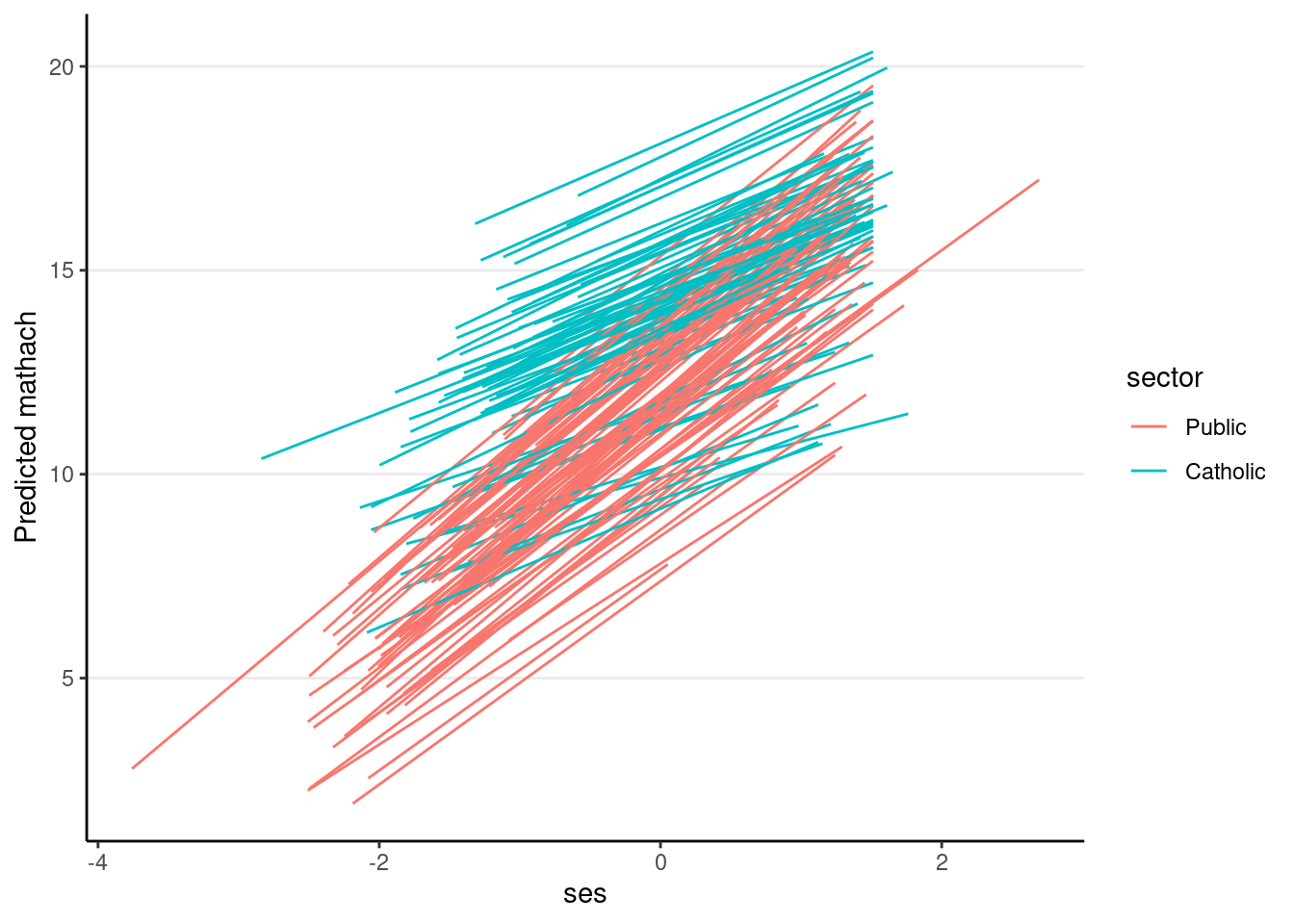

You can also use the sjPlot::plot_model() function for just the fixed effects:

plot_model(crlv_int, type = "pred", pred.type = "re",
           terms = c("ses_cmc", "id", "sector"),
           # suppress confidence band
           ci.lvl = NA, show.legend = FALSE, colors = "gs",
           # suppress title
           title = "",
           axis.title = c("SES (cluster-mean centered)", "Math Achievement"),
           show.data = TRUE, dot.size = 0.5, dot.alpha = 0.5)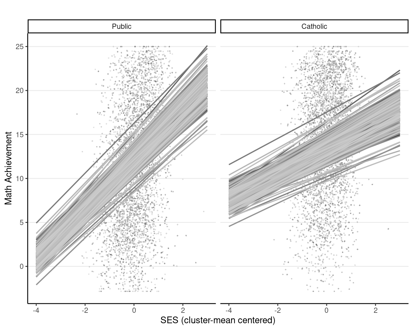

Summaizing Analyses in a Table

You can again use the msummary() function from the modelsummary package to quickly summarize the results in a table.

# Basic table from `modelsummary`
msummary(list(
    "Between-within" = m_bw,
    "Contextual" = contextual,
    "Random slope" = ran_slp,
    "Cross-level interaction" = crlv_int
))

	Between-within	Contextual	Random slope	Cross-level interaction
(Intercept)	12.648	12.661	12.645	12.085
	(0.149)	(0.149)	(0.149)	(0.199)
meanses	5.866	3.675	5.896	5.245
	(0.362)	(0.378)	(0.360)	(0.368)
ses_cmc	2.191		2.191	2.788
	(0.109)		(0.128)	(0.156)
ses		2.191
		(0.109)
sectorCatholic				1.252
				(0.306)
sectorCatholic × ses_cmc				−1.348
				(0.235)
SD (Intercept id)	1.641	1.641	1.641	1.543
SD (ses_cmc id)			0.828	0.521
Cor (Intercept~ses_cmc id)			−0.195	0.244
SD (Observations)	6.084	6.084	6.059	6.059
Num.Obs.	7185	7185	7185	7185
R2 Marg.	0.167	0.167	0.168	0.176
R2 Cond.	0.224	0.224	0.231	0.228
AIC	46578.6	46578.6	46571.7	46532.5
BIC	46613.0	46613.0	46619.8	46594.4
ICC	0.07	0.07	0.08	0.06
RMSE	6.03	6.03	5.99	6.00

Bonus: More “APA-like” Table

Make it look like the table at https://apastyle.apa.org/style-grammar-guidelines/tables-figures/sample-tables#regression. You can see a recent recommendation in this paper published in the Journal of Memory and Language

# Step 1. Create a map for the predictors and the terms in the model.
# Need to use '\\( \\)' to show math.
# Rename and reorder the rows. Need to use '\\( \\)' to
# show math. If this does not work for you, don't worry about it.
cm <- c("(Intercept)" = "Intercept",
        "meanses" = "school mean SES",
        "ses_cmc" = "SES (cluster-mean centered)",
        "sectorCatholic" = "Catholic school",
        "sectorCatholicses_cmc" = "Catholic school x SES (cmc)",
        "SD (Intercept id)" = "\\(\\tau_0\\)",
        "SD (ses_cmc id)" = "\\(\\tau_1\\) (SES)",
        "Cor (Intercept~ses_cmc id)" = "\\(\\tau_{01}\\)",
        "SD (Observations)" = "\\(\\sigma\\)")
# Step 2. Create a list of models to have one column for coef,
# one for SE, one for CI, and one for p
models <- list(
    "Estimate" = crlv_int,
    "SE" = crlv_int,
    "95% CI" = crlv_int
)
# Step 3. Add rows to say fixed and random effects
# (Need same number of columns as the table)
new_rows <- data.frame(
    term = c("Fixed effects", "Random effects"),
    est = c("", ""),
    se = c("", ""),
    ci = c("", "")
)
# Specify which rows to add
attr(new_rows, "position") <- c(1, 7)
# Step 4. Render the table
msummary(models,
         estimate = c("estimate", "std.error",
                      "[{conf.low}, {conf.high}]"),
         statistic = NULL,  # suppress the extra rows for SEs
         # suppress gof indices (e.g., R^2)
         gof_omit = ".*",
         coef_map = cm,
         add_rows = new_rows)

	Estimate	SE	95% CI
Fixed effects
Intercept	12.085	0.199	[11.695, 12.474]
school mean SES	5.245	0.368	[4.523, 5.967]
SES (cluster-mean centered)	2.788	0.156	[2.482, 3.093]
Catholic school	1.252	0.306	[0.652, 1.853]
$τ_{0}$	1.543
Random effects
$τ_{1}$ (SES)	0.521
$τ_{01}$	0.244
$σ$	6.059

Load Packages and Import Data

Import Data

Between-Within Decomposition

Cluster-mean centering

Model Equation

Running in R

Contextual Effect

Model Equation

Running in R

Random-Coefficients Model

Explore Variations in Slopes

Model Equation

Running in R

Showing the random intercepts and slopes

Plotting Random Slopes

Including the effect of meanses

Effect Size

Analyzing Cross-Level Interactions

Model Equation

Running in R

Effect Size

Simple Slopes

Plotting the Interactions

Summaizing Analyses in a Table

Bonus: More “APA-like” Table

Including the effect of `meanses`