Week 10 (R): Longitudinal II

Load Packages and Import Data

# To install a package, run the following ONCE (and only once on your computer)
# install.packages("psych")
library(here)  # makes reading data more consistent
library(tidyverse)  # for data manipulation and plotting
library(haven)  # for importing SPSS/SAS/Stata data
library(lme4)  # for multilevel analysis
library(glmmTMB)  # for frequentist longitudinal MLM

># Warning in checkMatrixPackageVersion(): Package version inconsistency detected.
># TMB was built with Matrix version 1.5.1
># Current Matrix version is 1.5.3
># Please re-install 'TMB' from source using install.packages('TMB', type = 'source') or ask CRAN for a binary version of 'TMB' matching CRAN's 'Matrix' package

library(brms)  # for Bayesian longitudinal MLM
library(sjPlot)  # for plotting
library(modelsummary)  # for making tables

# Read in the data from GitHub (need Internet access)
curran_wide <- read_sav("https://github.com/MultiLevelAnalysis/Datasets-third-edition-Multilevel-book/raw/master/chapter%205/Curran/CurranData.sav")
# Make id a factor
curran_wide  # print the data

# Using the new `tidyr::pivot_longer()` function
curran_long <- curran_wide %>%
    pivot_longer(
        c(anti1:anti4, read1:read4),  # variables that are repeated measures
        # Convert 8 columns to 3: 2 columns each for anti/read (.value), and
        # one column for time
        names_to = c(".value", "time"),
        # Extract the names "anti"/"read" from the names of the variables for the
        # value columns, and then the number to the "time" column
        names_pattern = "(anti|read)([1-4])",
        # Convert the "time" column to integers
        names_transform = list(time = as.integer)
    ) %>%
    mutate(time0 = time - 1)

Covariance Structure

Observed covariance matrix across time

curran_wide %>%
    select(read1:read4) %>%
    cov(use = "pair") %>%
    print(digits = 2)

>#       read1 read2 read3 read4
># read1  0.86  0.67  0.57  0.48
># read2  0.67  1.17  0.96  0.96
># read3  0.57  0.96  1.35  1.08
># read4  0.48  0.96  1.08  1.56

Implied covariance based on OLS (independence)

m0_ols <- lm(read ~ factor(time), data = curran_long)
diag(sigma(m0_ols), nrow = 4) %>%
    round(digits = 2)

>#      [,1] [,2] [,3] [,4]
># [1,] 1.09 0.00 0.00 0.00
># [2,] 0.00 1.09 0.00 0.00
># [3,] 0.00 0.00 1.09 0.00
># [4,] 0.00 0.00 0.00 1.09

Implied covariance based on random intercept MLM (compound symmetry)

brms

m0_ri <- brm(read ~ 0 + factor(time) + (1 | id),
    data = curran_long,
    file = "brms_cached_m_cs"
)
vc_m0_ri <- VarCorr(m0_ri)
(matrix(vc_m0_ri$id$sd[1, "Estimate"]^2, nrow = 4, ncol = 4) +
    diag(vc_m0_ri$residual__$sd[1, "Estimate"]^2, nrow = 4)) %>%
    print(digits = 2)

>#      [,1] [,2] [,3] [,4]
># [1,] 1.20 0.79 0.79 0.79
># [2,] 0.79 1.20 0.79 0.79
># [3,] 0.79 0.79 1.20 0.79
># [4,] 0.79 0.79 0.79 1.20

glmmTMB

m0_ri_tmb <- glmmTMB(read ~ factor(time) + (1 | id),
  data = curran_long,
  REML = TRUE
)
vc_m0_ri_tmb <- VarCorr(m0_ri_tmb)
(matrix(vc_m0_ri_tmb[[1]]$id[1, 1], nrow = 4, ncol = 4) +
  diag(attr(vc_m0_ri_tmb[[1]], "sc")^2, nrow = 4)) %>%
  print(digits = 2)

>#      [,1] [,2] [,3] [,4]
># [1,] 1.20 0.79 0.79 0.79
># [2,] 0.79 1.20 0.79 0.79
># [3,] 0.79 0.79 1.20 0.79
># [4,] 0.79 0.79 0.79 1.20

Implied covariance based on random-slope MLM (piecewise growth)

brms

piece <- function(x, node) {
    cbind(pmin(x, node),
          pmax(x - node, 0))
}
# Fit the piecewise growth model
m_pw <- brm(
    read ~ piece(time0, node = 1) + (piece(time0, node = 1) | id),
    data = curran_long,
    file = "brms_cached_m_pw",
    # increase adapt_delta as there was a divergent transition warning
    control = list(adapt_delta = 0.9)
)
vc_mpw <- VarCorr(m_pw)
# Covariance
(cbind(1, c(0, 1, 1, 1), c(0, 0, 1, 2)) %*%
    vc_mpw$id$cov[, "Estimate", ] %*%
    rbind(1, c(0, 1, 1, 1), c(0, 0, 1, 2)) +
    diag(vc_mpw$residual__$sd[1, "Estimate"]^2, nrow = 4)) %>%
    print(digits = 2)

>#      [,1] [,2] [,3] [,4]
># [1,] 0.86 0.65 0.63 0.61
># [2,] 0.65 1.19 1.01 1.08
># [3,] 0.63 1.01 1.39 1.28
># [4,] 0.61 1.08 1.28 1.72

glmmTMB

# Fit the piecewise growth model
m_pw_tmb <- glmmTMB(
    read ~ piece(time0, node = 1) +
        (piece(time0, node = 1) | id),
    data = curran_long, REML = TRUE,
    # The default optimizer did not converge; try optim
    control = glmmTMBControl(
      optimizer = optim,
      optArgs = list(method = "BFGS")
    )
)
vc_mpw_tmb <- VarCorr(m_pw_tmb)
# Covariance
(cbind(1, c(0, 1, 1, 1), c(0, 0, 1, 2)) %*%
    vc_mpw_tmb[[1]]$id[1:3, 1:3] %*%
    rbind(1, c(0, 1, 1, 1), c(0, 0, 1, 2)) +
    diag(attr(vc_mpw_tmb[[1]], "sc")^2, nrow = 4)) %>%
    print(digits = 2)

>#      [,1] [,2] [,3] [,4]
># [1,] 0.86 0.65 0.63  0.6
># [2,] 0.65 1.18 1.01  1.1
># [3,] 0.63 1.01 1.39  1.3
># [4,] 0.60 1.08 1.27  1.7

Autoregressive(1) Error Structure

Note: You need brms or glmmTMB for AR covariance structure.

From the piecewise model, add the AR(1) error structure:

brms

# Add the AR(1) structure
m_pw_ar1 <- brm(
    read ~ piece(time0, node = 1) + (piece(time0, node = 1) | id) +
        ar(time = time0, gr = id),
    data = curran_long,
    # increase adapt_delta as there was a divergent transition warning
    control = list(adapt_delta = 0.9),
    # Also need more iterations
    iter = 4000,
    file = "brms_cached_m_pw_ar1"
)
vc_mpw_ar1 <- VarCorr(m_pw_ar1)
# Extract also AR estimate
est_ar <- posterior_summary(m_pw_ar1, variable = "ar[1]")[, "Estimate"]
# Covariance
(cbind(1, c(0, 1, 1, 1), c(0, 0, 1, 2)) %*%
    vc_mpw_ar1$id$cov[, "Estimate", ] %*%
    rbind(1, c(0, 1, 1, 1), c(0, 0, 1, 2)) +
    vc_mpw_ar1$residual__$sd[1, "Estimate"] ^ 2 ^
        (abs(outer(0:3, Y = 0:3, FUN = "-")) + 1)) %>%
    print(digits = 2)

>#      [,1] [,2] [,3] [,4]
># [1,] 0.86  0.7 0.62 0.61
># [2,] 0.70  1.2 1.06 1.06
># [3,] 0.62  1.1 1.39 1.32
># [4,] 0.61  1.1 1.32 1.70

glmmTMB

# Add the AR(1) structure
m_pw_ar1_tmb <- glmmTMB(
    read ~ piece(time0, node = 1) + (piece(time0, node = 1) | id) +
        ar1(0 + factor(time) | id),
    dispformula = ~0,
    data = curran_long, REML = TRUE,
    # The default optimizer did not converge; try optim
    control = glmmTMBControl(
        optimizer = optim,
        optArgs = list(method = "BFGS")
    )
)
vc_mpw_ar1_tmb <- VarCorr(m_pw_ar1_tmb)
# Covariance
(cbind(1, c(0, 1, 1, 1), c(0, 0, 1, 2)) %*%
    vc_mpw_ar1_tmb[[1]]$id[1:3, 1:3] %*%
    rbind(1, c(0, 1, 1, 1), c(0, 0, 1, 2)) +
    unname(vc_mpw_ar1_tmb[[1]]$id.1[1:4, 1:4])) %>%
    print(digits = 2)

>#      [,1] [,2] [,3] [,4]
># [1,] 0.86 0.65 0.62  0.6
># [2,] 0.65 1.18 1.01  1.1
># [3,] 0.62 1.01 1.39  1.3
># [4,] 0.60 1.08 1.27  1.7

Inference of AR structure

\(H_0\): \(\rho = 0\)

brms

Consider whether the 95% CI contains 0

posterior_summary(m_pw_ar1, variable = "ar[1]")  # not significant

>#        Estimate Est.Error       Q2.5     Q97.5
># ar[1] 0.1198533 0.1426947 -0.1550658 0.4046144

glmmTMB

anova(m_pw_tmb, m_pw_ar1_tmb)  # Not statistically significant

Intensive Longitudinal Data

The data is the first wave of the Cognition, Health, and Aging Project.

# Download the data from
# https://www.pilesofvariance.com/Chapter8/SPSS/SPSS_Chapter8.zip, and put it
# into the "data_files" folder
zip_data <- here("data_files", "SPSS_Chapter8.zip")
if (!file.exists(zip_data)) {
    download.file(
        "https://www.pilesofvariance.com/Chapter8/SPSS/SPSS_Chapter8.zip",
        zip_data
    )
}
stress_data <- read_sav(
    unz(zip_data,
        "SPSS_Chapter8/SPSS_Chapter8.sav"))
stress_data

The data is already in long format.

Data Exploration

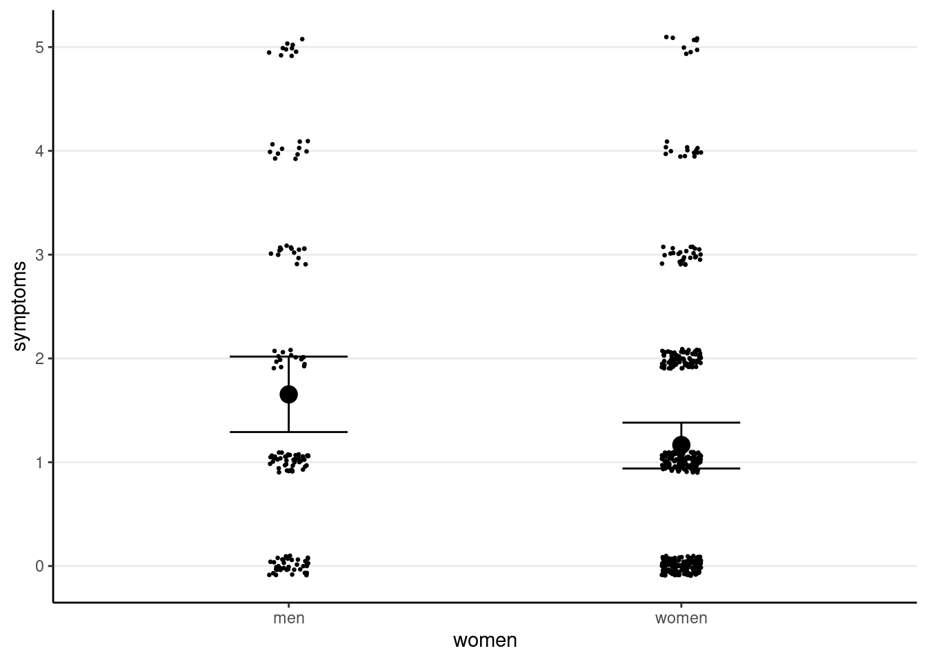
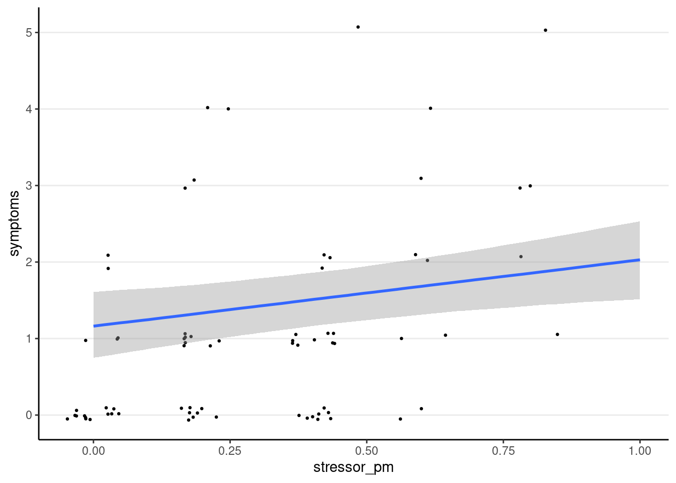
# First, separate the time-varying variables into within-person and
# between-person levels
stress_data <- stress_data %>%
    # Center mood (originally 1-5) at 1 for interpretation (so it becomes 0-4)
    # Also recode women to factor
    mutate(mood1 = mood - 1,
           women = factor(women, levels = c(0, 1),
                          labels = c("men", "women"))) %>%
    group_by(PersonID) %>%
    # The `across()` function applies the same procedure on
    # multiple variables
    mutate(across(c(symptoms, mood1, stressor),
                  # The `.` means the variable to be operated on
                  list("pm" = ~ mean(., na.rm = TRUE),
                       "pmc" = ~ . - mean(., na.rm = TRUE)))) %>%
    ungroup()
stress_data

# Use `datasummary_skim` for a quick summary
datasummary_skim(stress_data %>%
                     select(-PersonID, -session, -studyday, -dayofweek,
                            -weekend, -mood,
                            # PMC for a binary variable is not very meaningful
                            -stressor_pmc))

	Unique (#)	Missing (%)	Mean	SD	Min	Median	Max
baseage	103	0	80.1	6.1	69.7	80.0	95.3
symptoms	7	1	1.3	1.3	0.0	1.0	5.0
stressor	3	1	0.4	0.5	0.0	0.0	1.0
mood1	13	1	0.2	0.4	0.0	0.0	2.6
symptoms_pm	24	0	1.3	1.2	0.0	1.0	5.0
symptoms_pmc	44	1	−0.0	0.7	−2.4	0.0	3.0
mood1_pm	33	0	0.2	0.3	0.0	0.1	1.5
mood1_pmc	98	1	−0.0	0.3	−0.7	0.0	1.3
stressor_pm	8	0	0.4	0.3	0.0	0.4	1.0

stress_data %>%
    select(symptoms_pm, symptoms_pmc,
           mood1_pm, mood1_pmc, stressor_pm, stressor) %>%
    psych::pairs.panels(jiggle = TRUE, factor = 0.5, ellipses = FALSE,
                        cex.cor = 1, cex = 0.5)

Spaghetti Plot

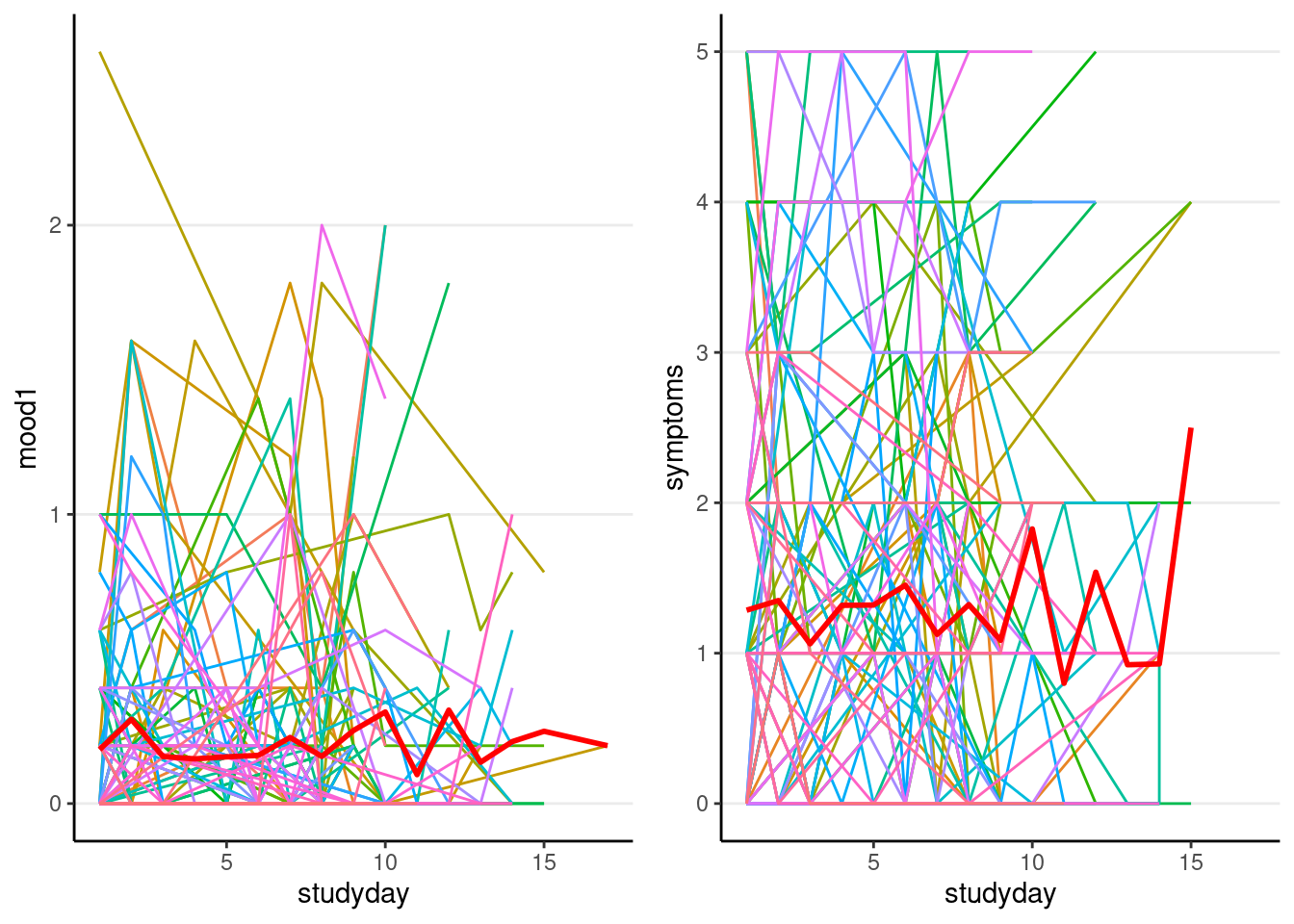
# Plotting mood
p1 <- ggplot(stress_data, aes(x = studyday, y = mood1)) +
    # add lines to connect the data for each person
    geom_line(aes(color = factor(PersonID), group = PersonID)) +
    # add a mean trajectory
    stat_summary(fun = "mean", col = "red", size = 1, geom = "line") +
    # suppress legend
    guides(color = "none")

># Warning: Using `size` aesthetic for lines was deprecated in ggplot2 3.4.0.
># ℹ Please use `linewidth` instead.

# Plotting symptoms
p2 <- ggplot(stress_data, aes(x = studyday, y = symptoms)) +
    # add lines to connect the data for each person
    geom_line(aes(color = factor(PersonID), group = PersonID)) +
    # add a mean trajectory
    stat_summary(fun = "mean", col = "red", size = 1, geom = "line") +
    # suppress legend
    guides(color = "none")
gridExtra::grid.arrange(p1, p2, ncol = 2)

># Warning: Removed 5 rows containing non-finite values (`stat_summary()`).

># Warning: Removed 3 rows containing missing values (`geom_line()`).

># Warning: Removed 6 rows containing non-finite values (`stat_summary()`).

># Warning: Removed 3 rows containing missing values (`geom_line()`).

We can see that there is not a clear trend across time but fluctuations.

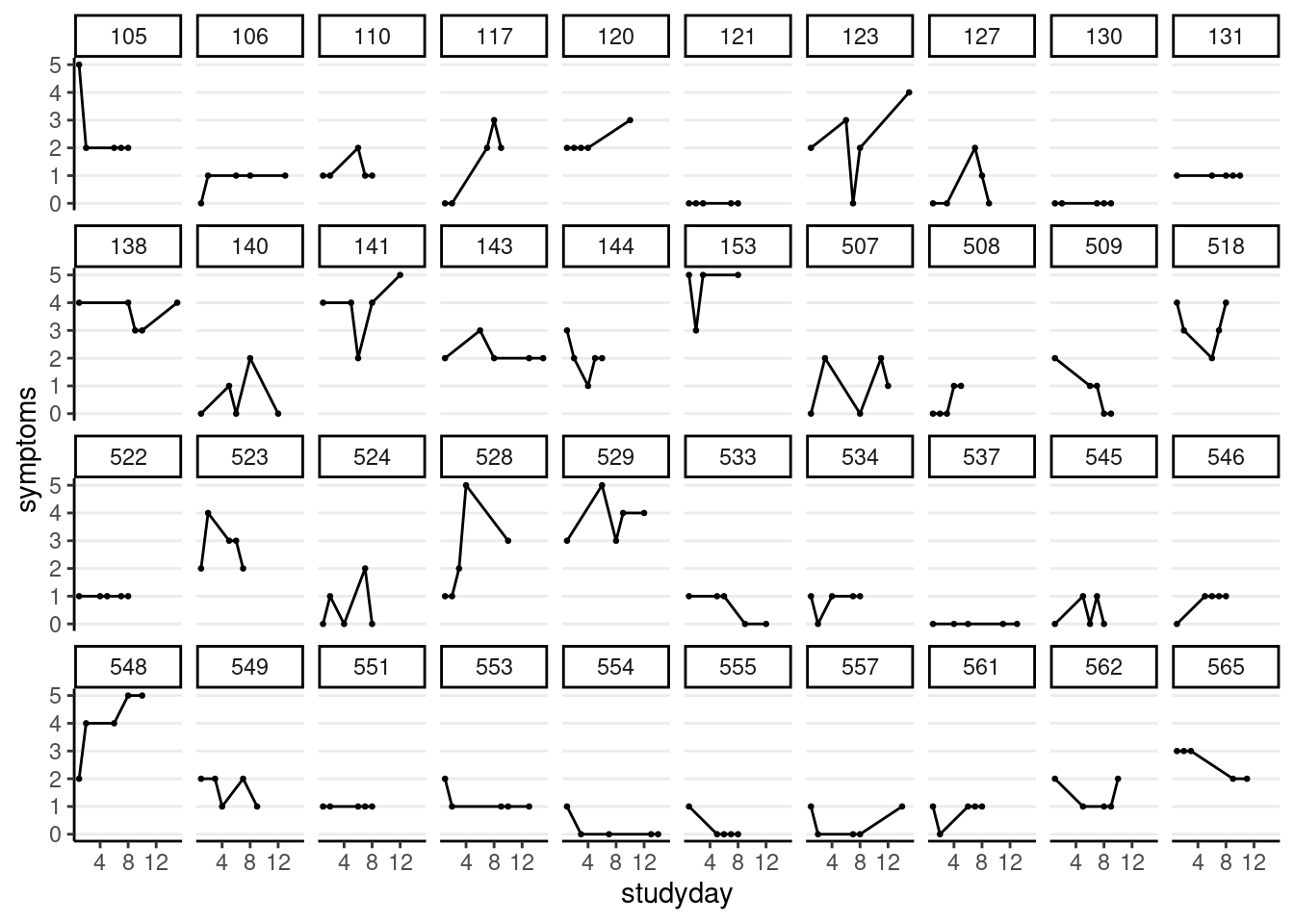
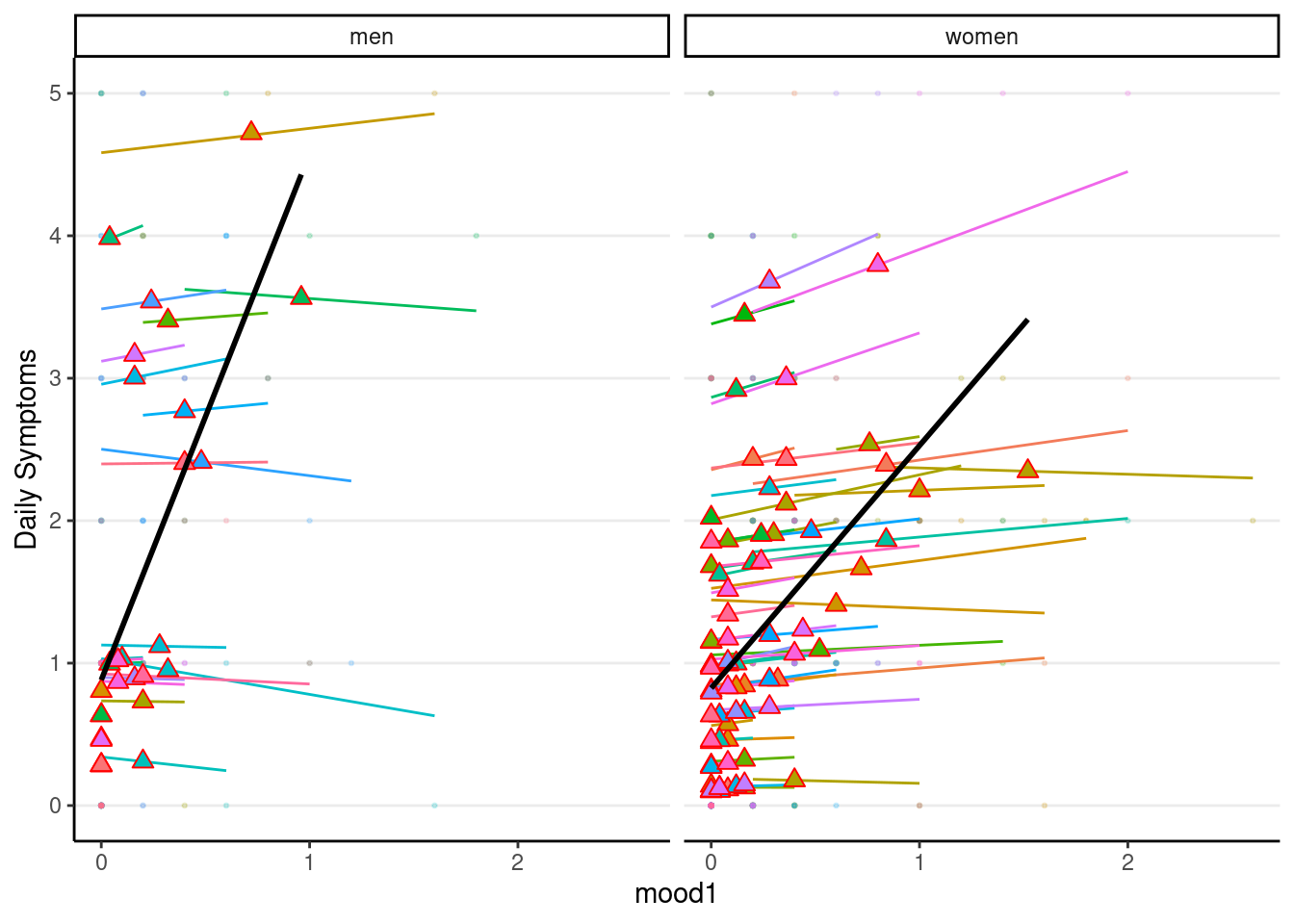
We can also plot the trajectories for a random sample of individuals:

stress_data %>%
    # randomly sample 40 individuals
    filter(PersonID %in% sample(unique(PersonID), 40)) %>%
    ggplot(aes(x = studyday, y = symptoms)) +
    geom_point(size = 0.5) +
    geom_line() +  # add lines to connect the data for each person
    facet_wrap(~ PersonID, ncol = 10)

># Warning: Removed 1 rows containing missing values (`geom_point()`).

Unconditional Models

The outcome is symptoms, and the time-varying predictors are mood1 and stressor. Let’s look at the ICC for each of them.

m0_symp <- lmer(symptoms ~ (1 | PersonID), data = stress_data)
performance::icc(m0_symp)

># # Intraclass Correlation Coefficient
># 
>#     Adjusted ICC: 0.668
>#   Unadjusted ICC: 0.668

m0_mood <- lmer(mood1 ~ (1 | PersonID), data = stress_data)
performance::icc(m0_mood)

># # Intraclass Correlation Coefficient
># 
>#     Adjusted ICC: 0.355
>#   Unadjusted ICC: 0.355

# Use glmer(..., family = binomial) for a binary outcome; to be discussed in a later week
m0_stre <- glmer(stressor ~ (1 | PersonID), data = stress_data,
                 family = binomial)
performance::icc(m0_stre)

># # Intraclass Correlation Coefficient
># 
>#     Adjusted ICC: 0.412
>#   Unadjusted ICC: 0.412

Check the Trend of the Data

One thing to consider with longitudinal data in a short time is whether there may be trends in the data due to contextual factors (e.g., weekend effect; shared life events at a specific time). If this is the case, a common practice is to de-trend the data; otherwise, associations between predictors and the outcome may be merely due to contextual factors happening on certain days.

There is no strong reason to think the data contain trends, as shown in the graphs. We can further test the linear trend:

m0_trend <- glmmTMB(symptoms ~ studyday + (studyday | PersonID),
    data = stress_data,
    REML = TRUE
)
summary(m0_trend)

>#  Family: gaussian  ( identity )
># Formula:          symptoms ~ studyday + (studyday | PersonID)
># Data: stress_data
># 
>#      AIC      BIC   logLik deviance df.resid 
>#   1487.4   1512.9   -737.7   1475.4      515 
># 
># Random effects:
># 
># Conditional model:
>#  Groups   Name        Variance Std.Dev. Corr  
>#  PersonID (Intercept) 1.238971 1.11309        
>#           studyday    0.002477 0.04977  -0.12 
>#  Residual             0.575147 0.75838        
># Number of obs: 519, groups:  PersonID, 105
># 
># Dispersion estimate for gaussian family (sigma^2): 0.575 
># 
># Conditional model:
>#              Estimate Std. Error z value Pr(>|z|)    
># (Intercept)  1.330849   0.125689  10.588   <2e-16 ***
># studyday    -0.005746   0.010817  -0.531    0.595    
># ---
># Signif. codes:  0 '***' 0.001 '**' 0.01 '*' 0.05 '.' 0.1 ' ' 1

which was not significant. If there was a trend, we should include the time variable when studying the time-varying covariates.

Covariance Structure

# Refit in glmmTMB
m0_symp <- glmmTMB(
    symptoms ~ (1 | PersonID),
    data = stress_data,
    REML = TRUE
)
# AR(1)
m0_ar1 <- glmmTMB(
    symptoms ~ ar1(factor(studyday) + 0 | PersonID),
    data = stress_data,
    REML = TRUE
)
anova(m0_symp, m0_ar1)  # not significant

Time-Varying Covariate

Aka level-1 predictors; also put in the cross-level interaction with women.

Level 1: \[\text{symptoms}_{ti} = \beta_{0i} + \beta_{1i} \text{mood1\_pmc}_{ti} + e_{ti}\] Level 2: \[ \begin{aligned} \beta_{0i} & = \gamma_{00} + \gamma_{01} \text{mood1\_pm}_{i} + \gamma_{02} \text{women}_i + \gamma_{03} \text{mood1\_pm}_{i} \times \text{women}_i + u_{0i} \\ \beta_{1i} & = \gamma_{10} + \gamma_{11} \text{women}_i + u_{1i} \end{aligned} \]

• \(\gamma_{03}\) = between-person interaction
• \(\gamma_{11}\) = cross-level interaction

m1 <- brm(
    symptoms ~ (mood1_pm + mood1_pmc) * women + (mood1_pmc | PersonID),
    data = stress_data,
    seed = 2315,
    file = "brms_cached_m1_symptoms"
)
summary(m1)

>#  Family: gaussian 
>#   Links: mu = identity; sigma = identity 
># Formula: symptoms ~ (mood1_pm + mood1_pmc) * women + (mood1_pmc | PersonID) 
>#    Data: stress_data (Number of observations: 514) 
>#   Draws: 4 chains, each with iter = 2000; warmup = 1000; thin = 1;
>#          total post-warmup draws = 4000
># 
># Group-Level Effects: 
># ~PersonID (Number of levels: 105) 
>#                          Estimate Est.Error l-95% CI u-95% CI Rhat Bulk_ESS
># sd(Intercept)                0.93      0.07     0.80     1.08 1.00     1005
># sd(mood1_pmc)                0.30      0.17     0.02     0.68 1.00     1278
># cor(Intercept,mood1_pmc)     0.44      0.39    -0.53     0.98 1.00     1986
>#                          Tail_ESS
># sd(Intercept)                1960
># sd(mood1_pmc)                1474
># cor(Intercept,mood1_pmc)     1494
># 
># Population-Level Effects: 
>#                      Estimate Est.Error l-95% CI u-95% CI Rhat Bulk_ESS
># Intercept                0.87      0.24     0.41     1.35 1.01      728
># mood1_pm                 3.82      0.83     2.22     5.53 1.00      894
># mood1_pmc                0.01      0.28    -0.53     0.57 1.00     2028
># womenwomen              -0.06      0.28    -0.61     0.48 1.01      627
># mood1_pm:womenwomen     -2.10      0.93    -3.96    -0.36 1.00      858
># mood1_pmc:womenwomen     0.16      0.33    -0.50     0.81 1.00     2002
>#                      Tail_ESS
># Intercept                1285
># mood1_pm                 1502
># mood1_pmc                2494
># womenwomen               1251
># mood1_pm:womenwomen      1329
># mood1_pmc:womenwomen     2358
># 
># Family Specific Parameters: 
>#       Estimate Est.Error l-95% CI u-95% CI Rhat Bulk_ESS Tail_ESS
># sigma     0.78      0.03     0.73     0.84 1.00     2898     2719
># 
># Draws were sampled using sampling(NUTS). For each parameter, Bulk_ESS
># and Tail_ESS are effective sample size measures, and Rhat is the potential
># scale reduction factor on split chains (at convergence, Rhat = 1).

Plotting

plot(
    conditional_effects(m1),
    points = TRUE,
    point_args = list(
        size = 0.5, width = 0.05, height = 0.1)
)

Between/Within effects

broom.mixed::augment(m1) %>%
    mutate(mood1 = mood1_pm + mood1_pmc) %>%
    ggplot(aes(x = mood1, y = symptoms, color = factor(PersonID))) +
    # Add points
    geom_point(size = 0.5, alpha = 0.2) +
    # Add within-cluster lines
    geom_smooth(aes(y = .fitted),
        method = "lm", se = FALSE, size = 0.5
    ) +
    # Add group means
    stat_summary(
        aes(x = mood1_pm, y = .fitted, fill = factor(PersonID)),
        color = "red", # add border
        fun = mean,
        geom = "point",
        shape = 24,
        # use triangles
        size = 2.5
    ) +
    # Add between coefficient
    geom_smooth(aes(x = mood1_pm, y = .fitted),
        method = "lm", se = FALSE,
        color = "black"
    ) +
    facet_grid(~women) +
    labs(y = "Daily Symptoms") +
    # Suppress legend
    guides(color = "none", fill = "none")

># `geom_smooth()` using formula = 'y ~ x'
># `geom_smooth()` using formula = 'y ~ x'

Add stressor

# Convert stressor to a factor
stress_data$stressor <- factor(stress_data$stressor,
                               levels = c(0, 1),
                               labels = c("stressor-free day", "stressor day"))
m2 <- brm(
    symptoms ~ (mood1_pm + mood1_pmc) * women + stressor_pm + stressor +
        (mood1_pmc + stressor | PersonID),
    data = stress_data,
    seed = 2315,
    file = "brms_cached_m2_symptoms"
)

Plotting

plot(
    conditional_effects(m2, effects = c("stressor_pm", "stressor")),
    points = TRUE,
    point_args = list(
        size = 0.5, width = 0.05, height = 0.1)
)

Bonus: Generalized Estimating Equations (GEE)

GEE is an alternative estimation method for clustered data, as discussed in 12.2 of Snijders and Bosker. It is a popular method, especially for longitudinal data in some research areas, as it offers some robustness against misspecification in the random effect structure (e.g., autoregressive errors, missing random slopes, etc). It accounts for the covariance structure using a working correlation matrix, such as the exchangeable (aka compound symmetry) structure. On the other hand, it only estimates fixed effects (also called marginal effects), so we cannot know whether some slopes are different across persons, but only the average slopes. GEE estimates the fixed effects by iteratively calculating the working correlation matrix and updating the fixed effect estimates with OLS. At the end, it computes the standard errors using the cluster-robust sandwich estimator.

GEE tends to require a relatively large sample size, and is usually less efficient than MLM for the same model (i.e., GEE gives larger standard errors, wider confidence intervals, and thus has less statistical power), which can be seen in the example below.

Below is a quick demonstration of GEE using the geepack package in R.

stress_data_lw <- stress_data %>%
    drop_na(mood1_pm, mood1_pmc, women, stressor_pm, stressor) %>%
    # Also need to convert to a data frame (instead of tibble)
    as.data.frame()

library(geepack)
m2_gee <- geeglm(symptoms ~ (mood1_pm + mood1_pmc) * women +
                   stressor_pm + stressor,
                 data = stress_data_lw,
                 id = PersonID,
                 corstr = "exchangeable",
                 std.err = "san.se")
summary(m2_gee)

># 
># Call:
># geeglm(formula = symptoms ~ (mood1_pm + mood1_pmc) * women + 
>#     stressor_pm + stressor, data = stress_data_lw, id = PersonID, 
>#     corstr = "exchangeable", std.err = "san.se")
># 
>#  Coefficients:
>#                      Estimate  Std.err   Wald Pr(>|W|)    
># (Intercept)           0.54884  0.22897  5.745 0.016531 *  
># mood1_pm              3.19491  0.91671 12.146 0.000492 ***
># mood1_pmc            -0.12724  0.25705  0.245 0.620613    
># womenwomen           -0.07326  0.27306  0.072 0.788486    
># stressor_pm           0.90373  0.32419  7.771 0.005309 ** 
># stressorstressor day  0.06741  0.09278  0.528 0.467476    
># mood1_pm:womenwomen  -1.89663  0.93949  4.076 0.043509 *  
># mood1_pmc:womenwomen  0.28588  0.29847  0.917 0.338155    
># ---
># Signif. codes:  0 '***' 0.001 '**' 0.01 '*' 0.05 '.' 0.1 ' ' 1
># 
># Correlation structure = exchangeable 
># Estimated Scale Parameters:
># 
>#             Estimate Std.err
># (Intercept)    1.323   0.152
>#   Link = identity 
># 
># Estimated Correlation Parameters:
>#       Estimate Std.err
># alpha   0.5207 0.04957
># Number of clusters:   105  Maximum cluster size: 5

# Small sample correction (Mancl & DeRouen, 2001) for the robust standard errors
library(geesmv)
m2_vcov_md <- GEE.var.md(symptoms ~ (mood1_pm + mood1_pmc) * women +
                           stressor_pm + stressor,
                         data = stress_data_lw,
                         id = "PersonID",  # need to be string
                         corstr = "exchangeable")

># Beginning Cgee S-function, @(#) geeformula.q 4.13 98/01/27

># running glm to get initial regression estimate

>#          (Intercept)             mood1_pm            mood1_pmc 
>#              0.56476              2.97820             -0.21094 
>#           womenwomen          stressor_pm stressorstressor day 
>#             -0.08227              0.88983              0.07183 
>#  mood1_pm:womenwomen mood1_pmc:womenwomen 
>#             -1.68409              0.37119

library(lmtest)  # For testing using corrected standard error

># Loading required package: zoo

># 
># Attaching package: 'zoo'

># The following objects are masked from 'package:base':
># 
>#     as.Date, as.Date.numeric

coeftest(m2_gee, diag(m2_vcov_md$cov.beta))

># 
># z test of coefficients:
># 
>#                      Estimate Std. Error z value Pr(>|z|)   
># (Intercept)            0.5488     0.2636    2.08   0.0373 * 
># mood1_pm               3.1949     1.3114    2.44   0.0148 * 
># mood1_pmc             -0.1272     0.3015   -0.42   0.6730   
># womenwomen            -0.0733     0.3104   -0.24   0.8134   
># stressor_pm            0.9037     0.3428    2.64   0.0084 **
># stressorstressor day   0.0674     0.0941    0.72   0.4738   
># mood1_pm:womenwomen   -1.8966     1.3428   -1.41   0.1578   
># mood1_pmc:womenwomen   0.2859     0.3417    0.84   0.4028   
># ---
># Signif. codes:  0 '***' 0.001 '**' 0.01 '*' 0.05 '.' 0.1 ' ' 1

# Ignore clustering
m2_lm <- lm(
    symptoms ~ (mood1_pm + mood1_pmc) * women +
        stressor_pm + stressor,
    data = stress_data_lw
)
# Refit m2 with glmmTMB
m2 <- lmer(
    symptoms ~ (mood1_pm + mood1_pmc) * women + stressor_pm + stressor +
        (mood1_pmc + stressor | PersonID),
    data = stress_data_lw
)

># boundary (singular) fit: see help('isSingular')

# Compare the fixed effects
msummary(
    list(
        OLS = m2_lm,
        MLM = m2,
        `GEE (Sandwich SE)` = m2_gee,
        `GEE (Sandwich SE + small-sample correction)` = m2_gee
    ),
    vcov = list(
        OLS = NULL,
        MLM = NULL,
        `GEE (Sandwich SE)` = NULL,
        `GEE (Sandwich SE + small-sample correction)` =
        diag(m2_vcov_md$cov.beta)
    ),
    coef_rename = c("mood1_pmwomenwomen" = "mood1_pm:womenwomen",
                    "mood1_pmcwomenwomen" = "mood1_pmc:womenwomen")
)

	OLS	MLM	GEE (Sandwich SE)	GEE (Sandwich SE + small-sample correction)
(Intercept)	0.565	0.452	0.549	0.549
	(0.144)	(0.236)	(0.229)	(0.229)
mood1_pm	2.978	3.438	3.195	3.195
	(0.468)	(0.784)	(0.917)	(0.917)
mood1_pmc	−0.211	−0.064	−0.127	−0.127
	(0.399)	(0.283)	(0.257)	(0.257)
womenwomen	−0.082	0.039	−0.073	−0.073
	(0.152)	(0.250)	(0.273)	(0.273)
stressor_pm	0.890	0.848	0.904	0.904
	(0.218)	(0.300)	(0.324)	(0.324)
stressorstressor day	0.072	0.064	0.067	0.067
	(0.142)	(0.100)	(0.093)	(0.093)
mood1_pm:womenwomen	−1.684	−1.958	−1.897	−1.897
	(0.506)	(0.856)	(0.939)	(0.939)
mood1_pmc:womenwomen	0.371	0.251	0.286	0.286
	(0.451)	(0.321)	(0.298)	(0.298)
SD (Intercept PersonID)		0.732
SD (mood1_pmc PersonID)		0.207
SD (stressorstressor day PersonID)		0.265
Cor (Intercept~mood1_pmc PersonID)		0.607
Cor (Intercept~stressorstressor day PersonID)		0.984
Cor (mood1_pmc~stressorstressor day PersonID)		0.738
SD (Observations)		0.781
Num.Obs.	513	513	513	513
R2	0.253		0.253	0.253
R2 Adj.	0.243
R2 Marg.		0.272
R2 Cond.		0.672
AIC	1616.9	1436.7	1617.3	1617.3
BIC	1655.1	1500.3	1655.4	1655.4
ICC		0.5
Log.Lik.	−799.450		−799.632	−799.632
RMSE	1.15	0.70	1.15	1.15
Std.Errors	OLS	MLM	GEE (Sandwich SE)	GEE (Sandwich SE + small-sample correction)

As shown above, for OLS regression, which ignores the temporal dependence of the data, the standard errors for the between-level coefficients are too small. The results with MLM and GEE are comparable, although GEE only gives fixed effect estimates. Overall, GEE tends to have larger standard errors, especially when using the small-sample correction. In sum, the pros and cons of GEE are:

• Pros:
  • Not requiring specification of the random part
  • Robust to moderate degree of misspecification in the random-effect covariance structure
  • Likely valid inferences on the fixed effects
• Cons:
  • Loss of statistical power (which may not be a concern in really large samples)
  • No results and predictions for individual-specific models, as the random effect part is not modeled
  • No likelihood-based statistical tools (e.g., AIC/BIC)