# To install a package, run the following ONCE (and only once on your computer)
# install.packages("psych")
library(here)  # makes reading data more consistent
library(tidyverse)  # for data manipulation and plotting
library(haven)  # for importing SPSS/SAS/Stata data
library(lme4)  # for multilevel analysis
library(lmerTest)  # for testing coefficients
library(MuMIn)  # for R^2
library(sjPlot)  # for plotting effects
library(emmeans)  # for marginal means
library(modelsummary) # for making tablesWeek 8 (R): MLM for Experiments
Load Packages and Import Data
This note focused on within-subjects experimental designs, as between-subjects designs are generally easier to handle with the treatment condition at the upper level. When clusters of people are randomly assigned, the design is called a cluster-randomized trial. See an example here: https://www.sciencedirect.com/science/article/abs/pii/S0022103117300860.
# Data example of Hoffman & Atchley (2001)
# Download from the Internet, unzip, and read in
zip_path <- here("data_files", "MLM_for_Exp_Appendices.zip")
if (!file.exists(zip_path)) {
    download.file(
        "http://www.lesahoffman.com/Research/MLM_for_Exp_Appendices.zip",
        zip_path
    )
}
driving_dat <- read_sav(unz(zip_path, "MLM_for_Exp_Appendices/Ex1.sav"))
# Convert `sex` and `oldage` to factor
# Note: also convert id and Item to factor (just for plotting)
driving_dat <- driving_dat %>%
    mutate(
        sex = as_factor(sex),
        oldage = factor(oldage,
            levels = c(0, 1),
            labels = c("Below Age 40", "Over Age 40")
        ),
        # id = factor(id),
        Item = factor(Item)
    )
# Show data
rmarkdown::paged_table(driving_dat)
With SPSS data, you can view the variable labels by
# Show the variable labels
cbind(
    map(driving_dat, attr, "label")
)
># [,1]
># id "Participant ID"
># sex "Participant Sex (0=men, 1=women)"
># age "Age"
># NAME NULL
># rt_sec "Response Time in Seconds"
># Item NULL
># meaning "Meaning Rating (0-5)"
># salience "Salience Rating (0-5)"
># lg_rt "Natural Log RT in Seconds"
># oldage NULL
># older "Copy of oldage to be treated as categorical"
># yrs65 "Years Over Age 65 (0=65)"
># c_mean "Centered Meaning (0=3)"
># c_sal "Centered Salience (0=3)"Wide and Long Format
The data we used here is in what is called a long format, where each row corresponds to a unique observation, and is required for MLM. More commonly, however, you may have data in a wide format, where each row records multiple observations for each person, as shown below.
# Show data
rmarkdown::paged_table(driving_wide)
As can be seen above, rt_sec1 to rt_sec80 are the responses to the 51 items. If your data are like the above, you need to convert it to a long format. In R, this can be achieved using the pivot_long() function, as part of tidyverse (in the tidyr package):
driving_wide %>%
    pivot_longer(
        cols = rt_sec1:rt_sec80, # specify the columns of repeated measures
        names_to = "Item", # name of the new column to create to indicate item id
        names_prefix = "rt_sec", # remove "rt_sec" from the item ID column
        values_to = "rt_sec", # name of new column containing the response
    ) %>%
    rmarkdown::paged_table()
Descriptive Statistics
Missing Data Rate for Response Time:
driving_dat %>%
    group_by(id) %>%
    summarise(n_missing = sum(is.na(rt_sec))) %>%
    ggplot(aes(x = n_missing)) +
    geom_bar()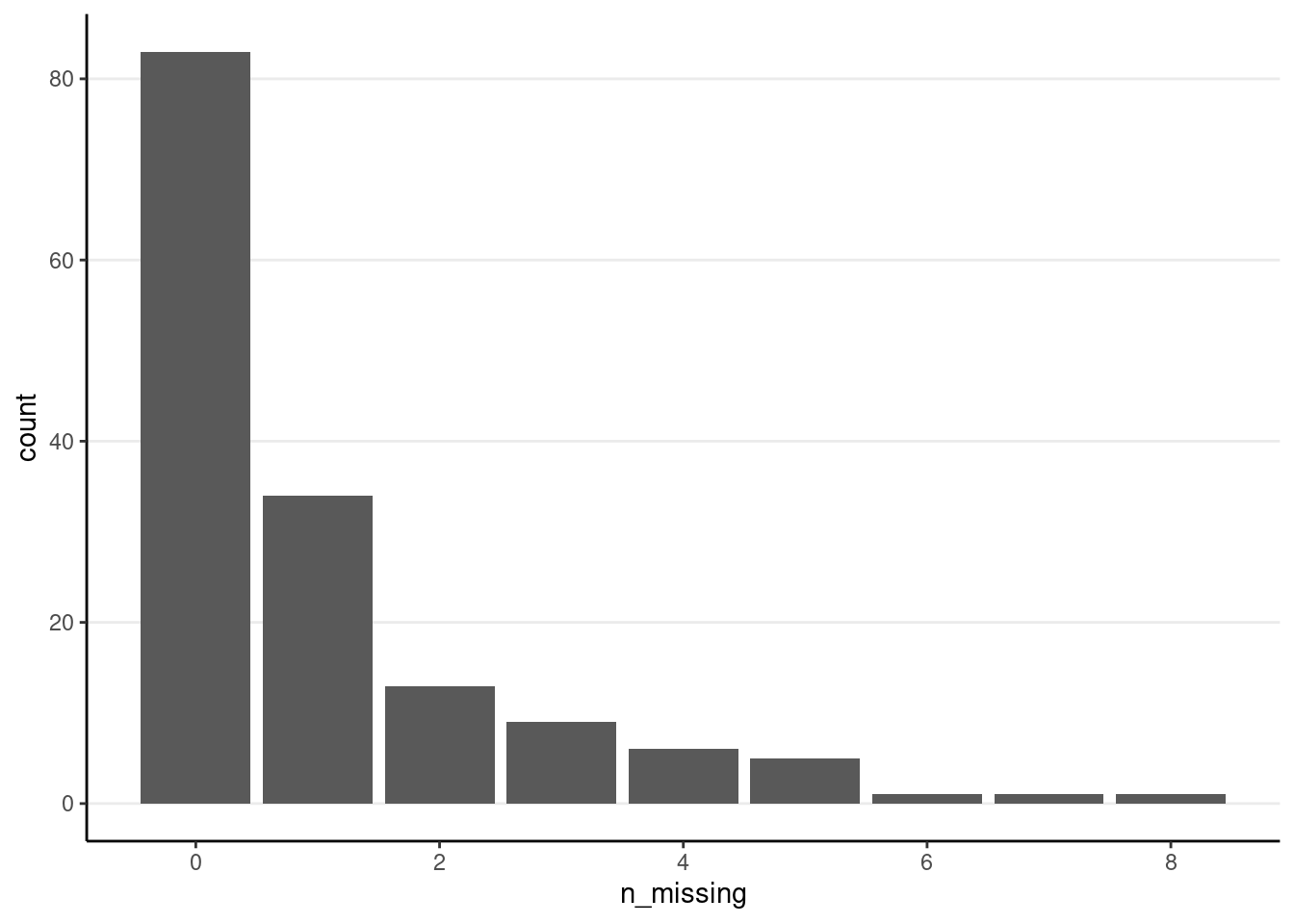
Note that only about 80 people have no missing data
Plotting
Let’s explore the data a bit with psych::pairs.panels().
driving_dat %>%
    # Select six variables
    select(sex, age, rt_sec, meaning, salience, lg_rt) %>%
    psych::pairs.panels(ellipses = FALSE, cex = 0.2, cex.cor = 1)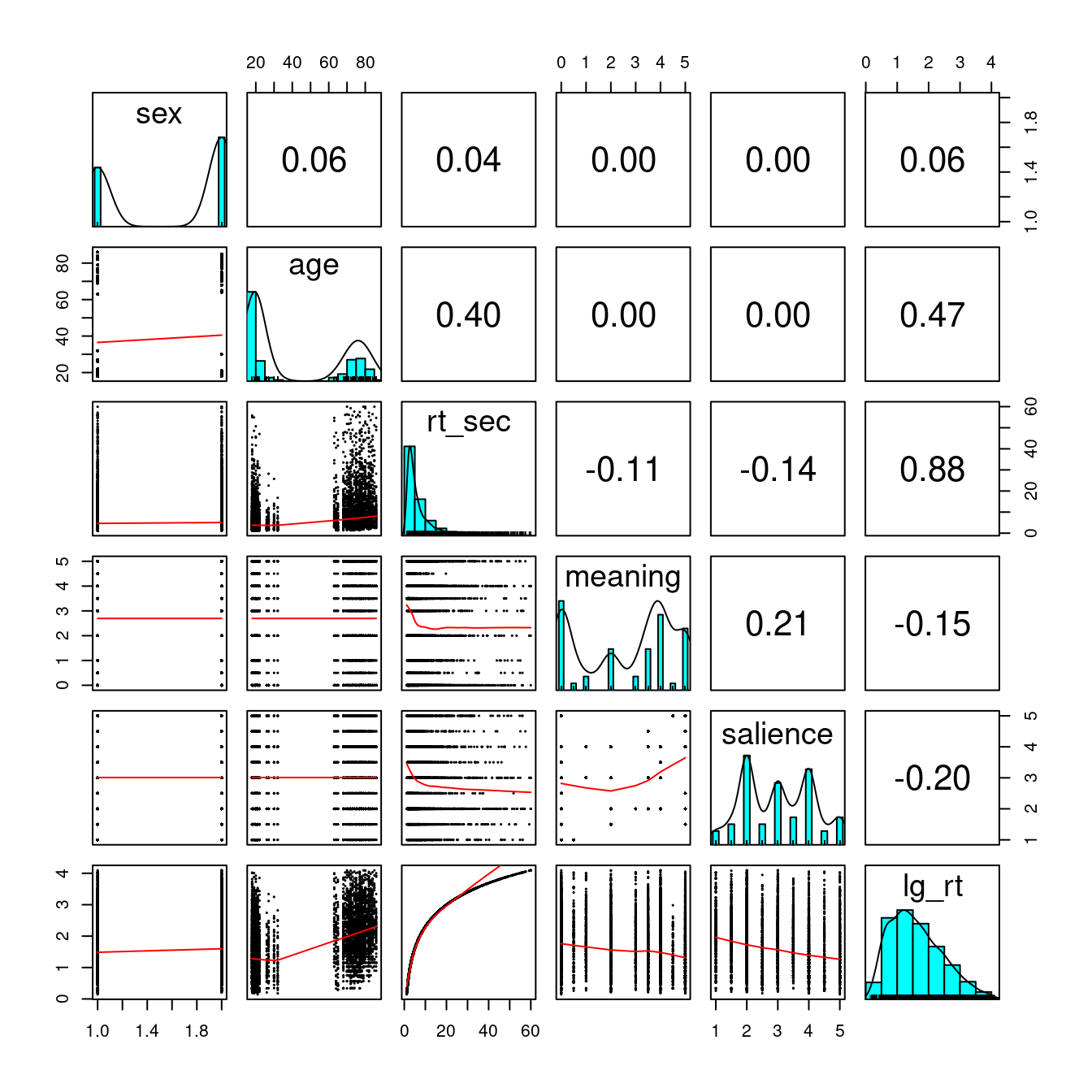
Note the nonnormality in response time. There doesn’t appear to be much gender differences.
Below is a plot between response time against age:
Left: original response time; Right: Natural log transformation
p1 <- driving_dat %>%
    ggplot(aes(x = age, y = rt_sec)) +
    geom_jitter(width = 0.5, height = 0, alpha = 0.5) +
    geom_smooth()
p2 <- driving_dat %>%
    ggplot(aes(x = age, y = lg_rt)) +
    geom_jitter(width = 0.5, height = 0, alpha = 0.5) +
    geom_smooth()
gridExtra::grid.arrange(p1, p2, ncol = 2)
># `geom_smooth()` using method = 'gam' and formula = 'y ~ s(x, bs = "cs")'># Warning: Removed 157 rows containing non-finite values (`stat_smooth()`).># Warning: Removed 157 rows containing missing values (`geom_point()`).># `geom_smooth()` using method = 'gam' and formula = 'y ~ s(x, bs = "cs")'># Warning: Removed 157 rows containing non-finite values (`stat_smooth()`).
># Removed 157 rows containing missing values (`geom_point()`).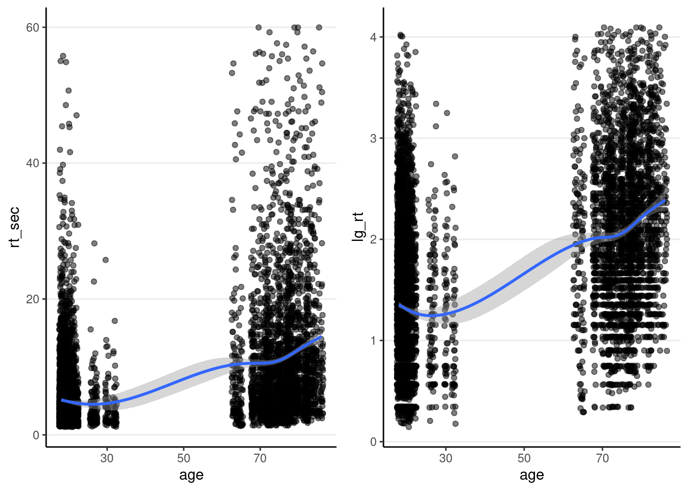
Cross-Classified Random Effect Analysis
Intraclass Correlations and Design Effects
Note: I used
lg_rtin the slides as the outcome variable, whereas here, I directly specify theloginsidelmer(). The two should give identical model fit and estimates. Usinglog(rt_sec)has the benefit of getting plots on the original response time variable; however, if you prefer plots on the log scale, you may want to uselg_rtinstead.
m0 <- lmer(log(rt_sec) ~ (1 | id) + (1 | Item), data = driving_dat)
vc_m0 <- as.data.frame(VarCorr(m0))
# ICC/Deff (person; cluster size = 51)
icc_person <- vc_m0$vcov[1] / sum(vc_m0$vcov)
# ICC (item; cluster size = 153)
icc_item <- vc_m0$vcov[2] / sum(vc_m0$vcov)
# ICC (person + item)
c("ICC(person + item)" = sum(vc_m0$vcov[1:2]) / sum(vc_m0$vcov))
># ICC(person + item)
># 0.4398793# For deff(person), need to take out the part for item
c("ICC(person)" = icc_person,
"Deff(person)" = (1 - icc_item) + (51 - 1) * icc_person)># ICC(person) Deff(person)
># 0.2589742 13.7678038# For deff(item), need to take out the part for person
c("ICC(item)" = icc_item,
"Deff(item)" = (1 - icc_person) + (153 - 1) * icc_item)># ICC(item) Deff(item)
># 0.1809051 28.2386059So both the item and the person levels are needed.
Visualizing person-level and item-level variances
set.seed(2124)
# Variation across persons
random_ids <- sample(unique(driving_dat$id), size = 15)
driving_dat %>%
    filter(id %in% random_ids) %>%  # select only 15 persons
    ggplot(aes(x = factor(id), y = lg_rt)) +
    geom_jitter(height = 0, width = 0.1, alpha = 0.3) +
    # Add person means
    stat_summary(fun = "mean", geom = "point", col = "red",
      shape = 17,  # use triangles
      size = 4  # make them larger
    ) +
    # change axis labels
    labs(x = "Person ID", y = "log(reaction time)")
># Warning: Removed 12 rows containing non-finite values (`stat_summary()`).># Warning: Removed 12 rows containing missing values (`geom_point()`).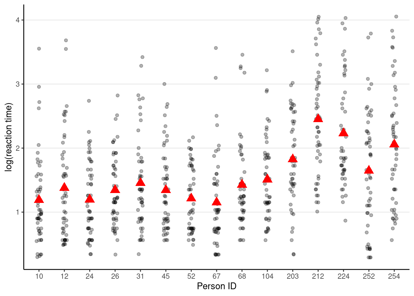
# Variation across items
random_items <- sample(unique(driving_dat$Item), size = 15)
driving_dat %>%
    filter(Item %in% random_items) %>%  # select only 15 items
    ggplot(aes(x = factor(Item), y = lg_rt)) +
    geom_jitter(height = 0, width = 0.1, alpha = 0.3) +
    # Add item means
    stat_summary(fun = "mean", geom = "point", col = "purple",
      shape = 17,  # use triangles
      size = 4  # make them larger
    ) +
    # change axis labels
    labs(x = "Item ID", y = "log(reaction time)")
># Warning: Removed 46 rows containing non-finite values (`stat_summary()`).># Warning: Removed 46 rows containing missing values (`geom_point()`).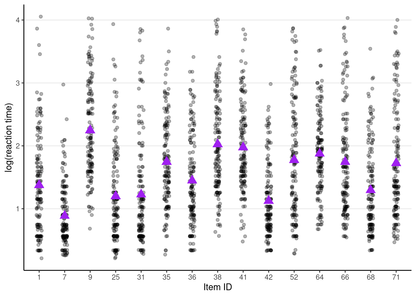
Now, it can be seen that
c_meanandc_salare item-level variables. The model is complex, but one thing that we don’t need to worry is that if the experimental design is balanced (i.e., every item was administered to every person), we don’t need to worry about cluster-means and cluster-mean centering. In this case,c_meanandc_salare purely item-level variables with no person-level variance. You can verify this:
lmer(c_mean ~ (1 | id), data = driving_dat)># boundary (singular) fit: see help('isSingular')># Linear mixed model fit by REML ['lmerModLmerTest']
># Formula: c_mean ~ (1 | id)
># Data: driving_dat
># REML criterion at convergence: 32061.49
># Random effects:
># Groups Name Std.Dev.
># id (Intercept) 0.000
># Residual 1.887
># Number of obs: 7803, groups: id, 153
># Fixed Effects:
># (Intercept)
># -0.3529
># optimizer (nloptwrap) convergence code: 0 (OK) ; 0 optimizer warnings; 1 lme4 warningsYou can see that the between-person variance for c_mean is zero. This, however, may not apply to unbalanced data, in which case cluster-means may still be needed.
Full Model
Equations
Repeated-Measure level (Lv 1): \[\log(\text{rt\_sec}_{i(j,k)}) = \beta_{0(j, k)} + e_{ijk}\] Between-cell (Person \(\times\) Item) level (Lv 2): \[\beta_{0(j, k)} = \gamma_{00} + \beta_{1j} \text{meaning}_{k} + \beta_{2j} \text{salience}_{k} + \beta_{3j} \text{meaning}_{k} \times \text{salience}_{k} + \beta_{4k} \text{oldage}_{j} + u_{0j} + v_{0k}\] Person level (Lv 2a) random slopes \[ \begin{aligned} \beta_{1j} = \gamma_{10} + \gamma_{11} \text{oldage}_{j} + u_{1j} \\ \beta_{2j} = \gamma_{20} + \gamma_{21} \text{oldage}_{j} + u_{2j} \\ \beta_{3j} = \gamma_{30} + \gamma_{31} \text{oldage}_{j} + u_{3j} \\ \end{aligned} \] Item level (Lv2b) random slopes \[\beta_{4k} = \gamma_{40} + v_{4k}\] Combined equations \[ \begin{aligned} \log(\text{rt\_sec}_{i(j,k)}) & = \gamma_{00} \\ & + \gamma_{10} \text{meaning}_{k} + \gamma_{20} \text{salience}_{k} + \gamma_{30} \text{meaning}_{k} \times \text{salience}_{k} + \gamma_{40} \text{oldage}_{j} \\ & + \gamma_{11} \text{meaning}_{k} \times \text{oldage}_{j} + \gamma_{21} \text{salience}_{k} \times \text{oldage}_{j} + \gamma_{31} \text{meaning}_{k} \times \text{oldage}_{j} \times \text{oldage}_{j} + \\ & + u_{0j} + u_{1j} \text{meaning}_{k} + u_{2j} \text{salience}_{k} + u_{3j} \text{meaning}_{k} \times \text{salience}_{k} \\ & + v_{0k} + v_{4k} \text{oldage}_{j} \\ & + e_{ijk} \end{aligned} \]
Testing random slopes
The random slopes can be tested one by one:
# First, no random slopes
m1 <- lmer(log(rt_sec) ~ c_mean * c_sal * oldage + (1 | id) + (1 | Item),
           data = driving_dat)
# Then test random slopes one by one
# Random slopes of oldage (person-level) across items
m1_rs1 <- lmer(
    log(rt_sec) ~ c_mean * c_sal * oldage + (1 | id) + (oldage | Item),
    data = driving_dat
)
# Test (see the line that says "oldage in (oldage | Item)")
ranova(m1_rs1)  # statistically significant, indicating varying slopes of
# oldage
# Random slopes of c_mean (item-level) across persons
m1_rs2 <- lmer(log(rt_sec) ~ c_mean * c_sal * oldage + (c_mean:c_sal | id) +
(1 | Item),
data = driving_dat)># boundary (singular) fit: see help('isSingular')# Test (see the line that says "c_mean:c_sal in (c_mean:c_sal | id)")
ranova(m1_rs2) # not statistically significant># boundary (singular) fit: see help('isSingular')# Random slopes of c_mean (item-level) across persons
m1_rs3 <- lmer(
log(rt_sec) ~ c_mean * c_sal * oldage + (c_mean | id) + (1 | Item),
data = driving_dat
)
# Test
ranova(m1_rs3) # not statistically significant># boundary (singular) fit: see help('isSingular')# Random slopes of c_sal (item-level) across persons
m1_rs4 <- lmer(
log(rt_sec) ~ c_mean * c_sal * oldage + (c_sal | id) + (1 | Item),
data = driving_dat
)
# Test
ranova(m1_rs4) # statistically significantSo the final model should include random slopes of oldage (a person-level predictor) across items and c_sal (an item-level predictor) across persons.
m1_rs <- lmer(log(rt_sec) ~ c_mean * c_sal * oldage +
                  (c_sal | id) + (oldage | Item),
              data = driving_dat)
# There was a convergence warning for the above model, but running
# `lme4::allFit()` shows that other optimizers gave the same results
# LRT for three-way interaction (not significant)
confint(m1_rs, parm = "c_mean:c_sal:oldageOver Age 40")
># Computing profile confidence intervals ...># 2.5 % 97.5 %
># c_mean:c_sal:oldageOver Age 40 -0.05341516 0.004624211# Dropping non-sig 3-way interaction
m2_rs <- lmer(log(rt_sec) ~ (c_mean + c_sal + oldage)^2 + (c_sal | id) +
(oldage | Item),
data = driving_dat)
# Compare model with and without two-way interactions
m3_rs <- lmer(log(rt_sec) ~ c_mean + c_sal + oldage + (c_sal | id) +
(oldage | Item),
data = driving_dat)># Warning in checkConv(attr(opt, "derivs"), opt$par, ctrl = control$checkConv, :
># Model failed to converge with max|grad| = 0.00231401 (tol = 0.002, component 1)anova(m2_rs, m3_rs) # LRT not significant># refitting model(s) with ML (instead of REML)# So we keep the additive model (i.e., no interaction)Coefficients
msummary(
    list(additive = m3_rs,
         `3-way interaction` = m1_rs),
    # Need the following when there are more than two levels
group = group + term ~ model)| additive | 3-way interaction | ||
|---|---|---|---|
| (Intercept) | 1.307 | 1.304 | |
| (0.049) | (0.051) | ||
| c_mean | −0.051 | −0.064 | |
| (0.023) | (0.025) | ||
| c_sal | −0.131 | −0.142 | |
| (0.041) | (0.044) | ||
| oldageOver Age 40 | 0.806 | 0.830 | |
| (0.044) | (0.044) | ||
| c_mean × c_sal | −0.003 | ||
| (0.021) | |||
| c_mean × oldageOver Age 40 | 0.038 | ||
| (0.018) | |||
| c_sal × oldageOver Age 40 | 0.012 | ||
| (0.033) | |||
| c_mean × c_sal × oldageOver Age 40 | −0.024 | ||
| (0.015) | |||
| id | SD (Intercept id) | 0.167 | 0.167 |
| SD (c_sal id) | 0.048 | 0.048 | |
| Cor (Intercept~c_sal id) | 0.030 | 0.032 | |
| Item | SD (Intercept Item) | 0.317 | 0.320 |
| SD (oldageOver Age 40 Item) | 0.223 | 0.210 | |
| Cor (Intercept~oldageOver Age 40 Item) | −0.274 | −0.279 | |
| Residual | SD (Observations) | 0.613 | 0.613 |
| Num.Obs. | 7646 | 7646 | |
| R2 Marg. | 0.266 | 0.270 | |
| R2 Cond. | 0.460 | 0.463 | |
| AIC | 39452.8 | 39476.4 | |
| BIC | 39529.1 | 39580.5 | |
| ICC | 0.3 | 0.3 | |
| RMSE | 0.60 | 0.60 |
Plot the 3-way interaction
Even though the 3-way interaction was not statistically significant, given that it was part of the prespecified hypothesis, let’s plot it
Note: the graphs here are based on the original response time (i.e., before log transformation), so they look different from the ones in the slides, which plotted the y-axis on the log scale.
plot_model(m1_rs, type = "int",
           show.data = TRUE, jitter = 0.1,
           dot.alpha = 0.5, dot.size = 0.2)
># Model has log-transformed response. Back-transforming predictions to
># original response scale. Standard errors are still on the log-scale.
># Model has log-transformed response. Back-transforming predictions to
># original response scale. Standard errors are still on the log-scale.
># Model has log-transformed response. Back-transforming predictions to
># original response scale. Standard errors are still on the log-scale.
># Model has log-transformed response. Back-transforming predictions to
># original response scale. Standard errors are still on the log-scale.># [[1]]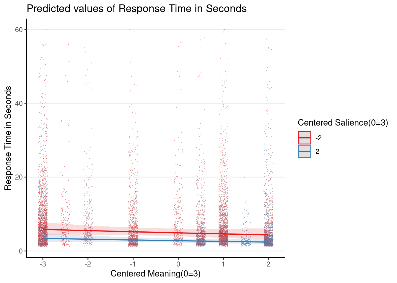
>#
># [[2]]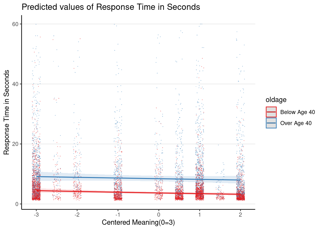
>#
># [[3]]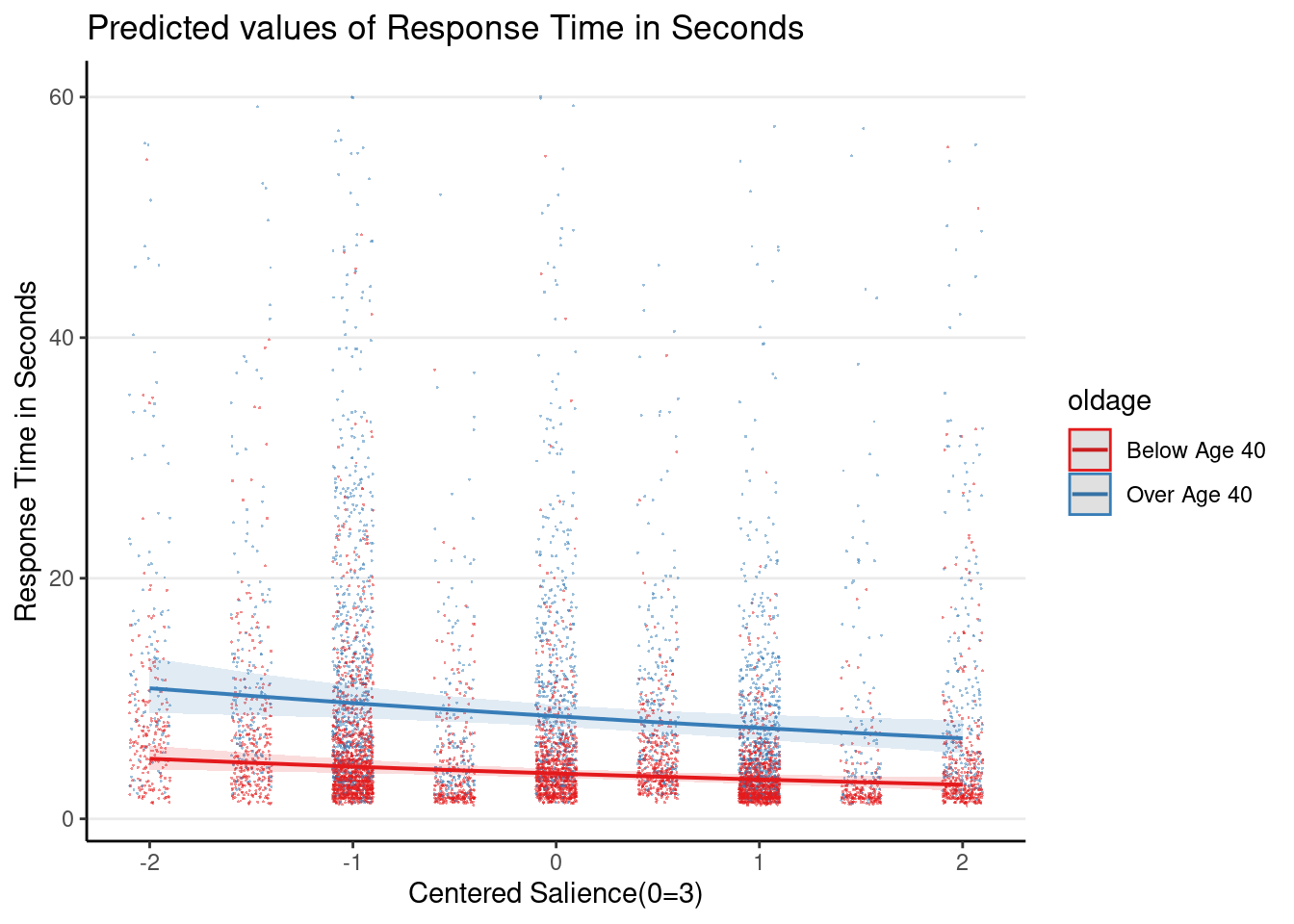
>#
># [[4]]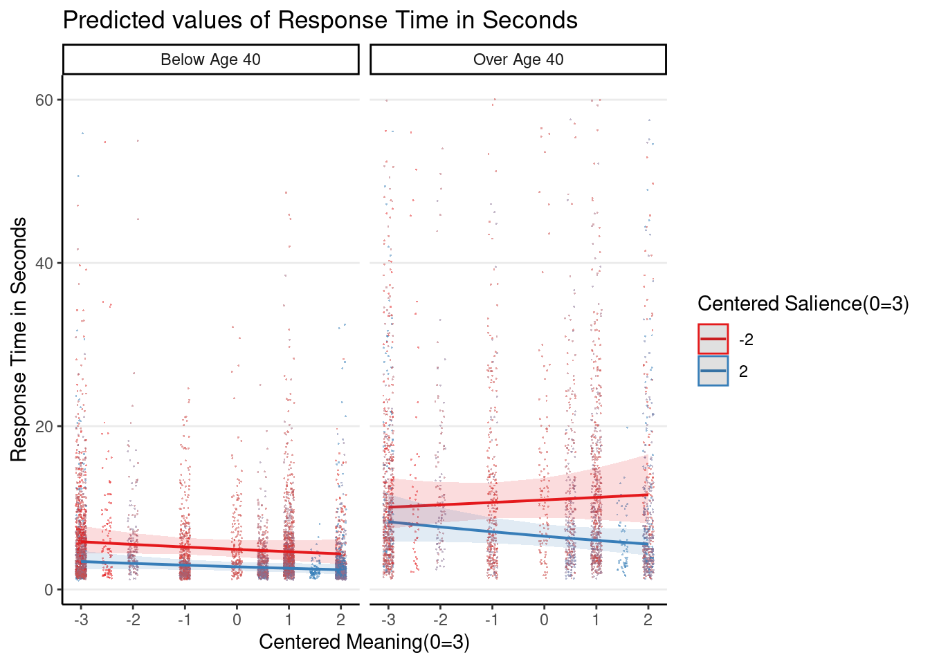
Plot the marginal age effect
# plot_model() function is from the `sjPlot` package
plot_model(m3_rs,
    type = "pred", terms = "c_mean",
    show.data = TRUE, jitter = 0.1,
    dot.alpha = 0.5, dot.size = 0.1
)
># Model has log-transformed response. Back-transforming predictions to
># original response scale. Standard errors are still on the log-scale.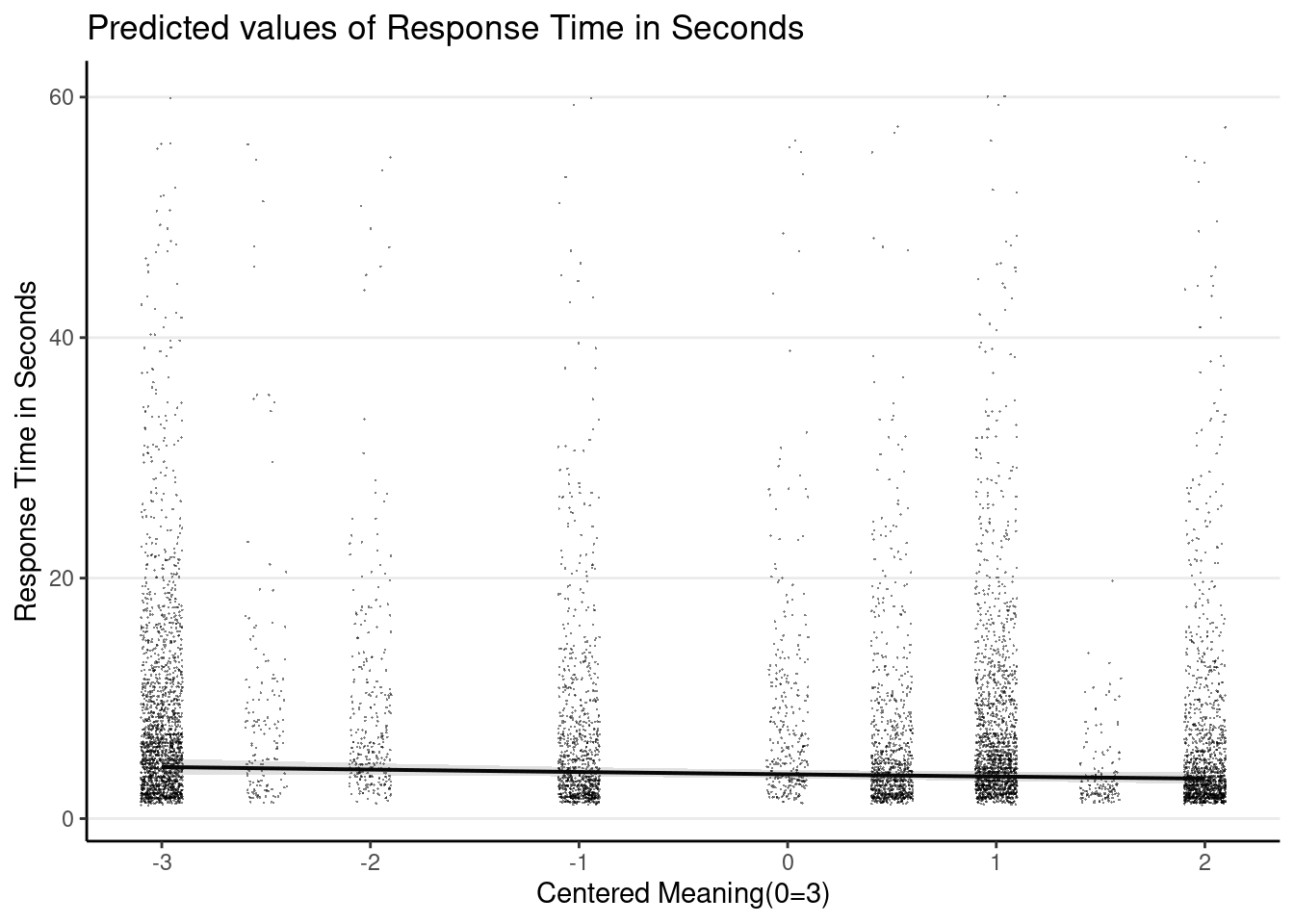
# Plot random slopes
plot_model(m3_rs,
    type = "pred",
    terms = c("c_sal", "id [1:274]"),
    pred.type = "re", show.legend = FALSE,
    colors = "black", line.size = 0.3,
    show.data = TRUE, jitter = 0.1,
    dot.alpha = 0.5, dot.size = 0.1,
    # suppress confidence band
    ci.lvl = NA
)
># Model has log-transformed response. Back-transforming predictions to
># original response scale. Standard errors are still on the log-scale.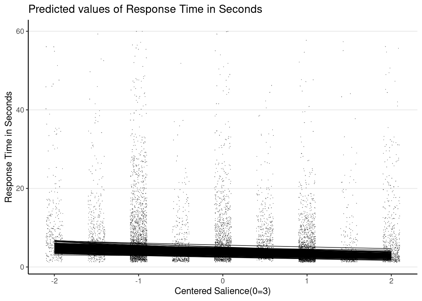
# Plot first 15 items
plot_model(m3_rs,
    type = "pred",
    terms = c("Item [1:15]", "oldage"),
    pred.type = "re"
) +
    theme(legend.position = "top")
># Model has log-transformed response. Back-transforming predictions to
># original response scale. Standard errors are still on the log-scale.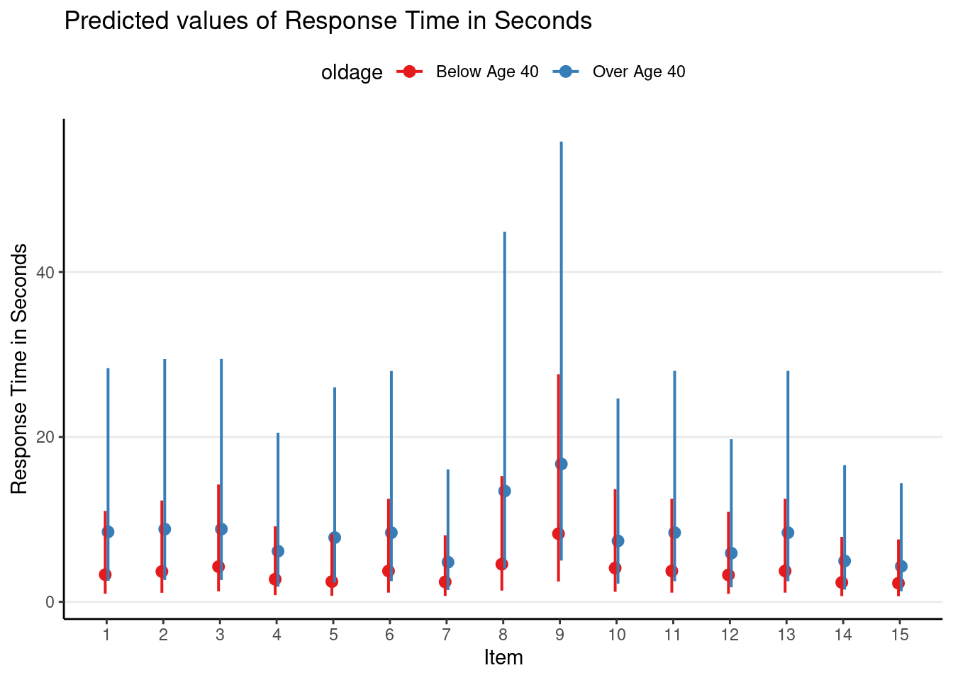
Predicted Value for Specified Conditions
When reporting results, one thing that students or researchers usually want to get is model predictions for different experimental conditions. With our example, there were three predictors, so we can get predictions for various value combinations on the three predictors. For example, one may be interested in the following levels:
c_mean: -3 vs. 2c_sal: -2 vs. 2oldage: Below Age 40 vs. Over Age 40
You can obtain predictions with the equations, which is usually the most reliable way in many cases (as long as you double and triple-check your calculations). However, with lme4, you can also use the predict() function and specify a data frame with all the combinations.
# Create data frame for prediction;
# the `crossing()` function generates all combinations of the input levels
pred_df <- crossing(
    c_mean = c(-3, 2),
    c_sal = c(-2, 2),
    oldage = c("Below Age 40", "Over Age 40")
)
# Add predicted values (log rt)
pred_df %>%
    mutate(
        .predicted = predict(m3_rs,
            # "newdata = ." means using the current data
            newdata = .,
            # "re.form = NA" means to not use random effects for prediction
            re.form = NA
        )
    )
Marginal Means
While the predict() function is handy, it requires users to specify values for each predictor. Sometimes researchers may simply be interested in the predicted means for levels of one or two predictors, while averaging across other predictors in the model. When averaging across one or more variables, the predicted means are usually called the marginal means. In this case, the emmeans package will be handy.
For example, suppose we are interested in only the marginal means for those below age 40 and those above age 40. We can use the following:
(emm_m3_rs <- emmeans(m3_rs, specs = "oldage", weights = "cell"))># Note: D.f. calculations have been disabled because the number of observations exceeds 3000.
># To enable adjustments, add the argument 'pbkrtest.limit = 7646' (or larger)
># [or, globally, 'set emm_options(pbkrtest.limit = 7646)' or larger];
># but be warned that this may result in large computation time and memory use.># Note: D.f. calculations have been disabled because the number of observations exceeds 3000.
># To enable adjustments, add the argument 'lmerTest.limit = 7646' (or larger)
># [or, globally, 'set emm_options(lmerTest.limit = 7646)' or larger];
># but be warned that this may result in large computation time and memory use.># oldage emmean SE df asymp.LCL asymp.UCL
># Below Age 40 1.32 0.0484 Inf 1.23 1.42
># Over Age 40 2.13 0.0530 Inf 2.02 2.23
>#
># Degrees-of-freedom method: asymptotic
># Results are given on the log (not the response) scale.
># Confidence level used: 0.95# Plotting the means
plot(emm_m3_rs)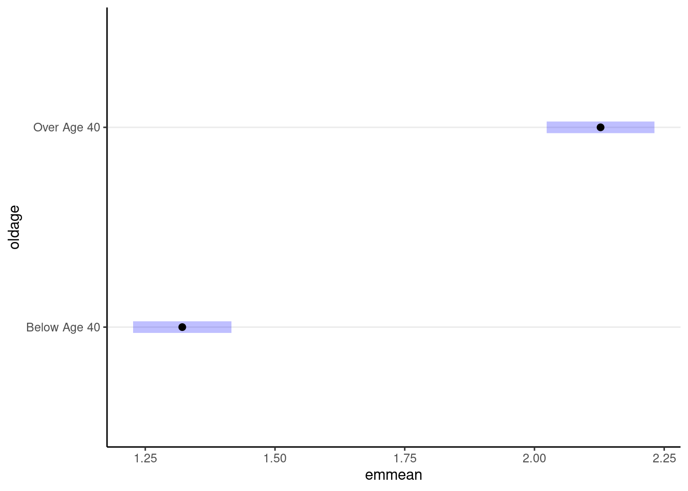
You can also obtain the marginal means for the transformed response variable. For example, because our response variable is log(rt), we can get the marginal means for the original response time variable:
emmeans(m3_rs, specs = "oldage", weights = "cell", type = "response")># Note: D.f. calculations have been disabled because the number of observations exceeds 3000.
># To enable adjustments, add the argument 'pbkrtest.limit = 7646' (or larger)
># [or, globally, 'set emm_options(pbkrtest.limit = 7646)' or larger];
># but be warned that this may result in large computation time and memory use.># Note: D.f. calculations have been disabled because the number of observations exceeds 3000.
># To enable adjustments, add the argument 'lmerTest.limit = 7646' (or larger)
># [or, globally, 'set emm_options(lmerTest.limit = 7646)' or larger];
># but be warned that this may result in large computation time and memory use.># oldage response SE df asymp.LCL asymp.UCL
># Below Age 40 3.75 0.181 Inf 3.41 4.12
># Over Age 40 8.39 0.445 Inf 7.56 9.31
>#
># Degrees-of-freedom method: asymptotic
># Confidence level used: 0.95
># Intervals are back-transformed from the log scaleEffect Size
You can compute \(R^2\). Using the additive model, the overall \(R^2\) is
MuMIn::r.squaredGLMM(m3_rs)># Warning: 'r.squaredGLMM' now calculates a revised statistic. See the help page.># R2m R2c
># [1,] 0.2661333 0.4603116# Alternatively
performance::r2(m3_rs)># # R2 for Mixed Models
>#
># Conditional R2: 0.460
># Marginal R2: 0.266With counterbalancing, the item-level (c_mean and c_sal) and the person-level (oldage) predictors are orthogonal, so we can get an \(R^2\) for the item-level predictors and an \(R^2\) for the person-level predictor, and they should add up approximately to the total \(R^2\). For example:
# Person-level (oldage)
m3_rs_oldage <- lmer(log(rt_sec) ~ oldage + (1 | id) +
                       (oldage | Item), data = driving_dat)
r.squaredGLMM(m3_rs_oldage)
># R2m R2c
># [1,] 0.2168664 0.4550552# Item-level (salience + meaning)
m3_rs_sal_mean <- lmer(log(rt_sec) ~ c_sal + c_mean + (c_sal | id) +
(1 | Item), data = driving_dat)
r.squaredGLMM(m3_rs_sal_mean)># R2m R2c
># [1,] 0.05162392 0.4465113The two above add up close to the total \(R^2\). However, c_sal and c_mean are positively correlated, so their individual contributions to the \(R^2\) would not add up to the value when both are included (as there is some overlap in their individual \(R^2\)). In this case, you can still report the individual \(R^2\), but also remember to report the total.
# Salience only
m3_rs_sal <- lmer(log(rt_sec) ~ c_sal + (c_sal | id) +
                         (1 | Item), data = driving_dat)
># Warning in checkConv(attr(opt, "derivs"), opt$par, ctrl = control$checkConv, :
># Model failed to converge with max|grad| = 0.00463405 (tol = 0.002, component 1)r.squaredGLMM(m3_rs_sal)># R2m R2c
># [1,] 0.03857116 0.4451035# Meaning only
m3_rs_mean <- lmer(log(rt_sec) ~ c_mean + (1 | id) +
(1 | Item), data = driving_dat)
r.squaredGLMM(m3_rs_mean)># R2m R2c
># [1,] 0.02353606 0.4414036As a note, the \(R^2\)s presented above are analogous to the \(\eta^2\) effect sizes in ANOVA.
Diagnostics
Marginal model plots
# Some discrepancy can be seen for `c_sal`
plot_model(m3_rs, type = "slope", show.data = TRUE)
># `geom_smooth()` using formula = 'y ~ x'
># `geom_smooth()` using formula = 'y ~ x'># Warning in simpleLoess(y, x, w, span, degree = degree, parametric =
># parametric, : pseudoinverse used at 0.995># Warning in simpleLoess(y, x, w, span, degree = degree, parametric =
># parametric, : neighborhood radius 1.005># Warning in simpleLoess(y, x, w, span, degree = degree, parametric =
># parametric, : reciprocal condition number 3.4597e-30># Warning in simpleLoess(y, x, w, span, degree = degree, parametric =
># parametric, : There are other near singularities as well. 1.01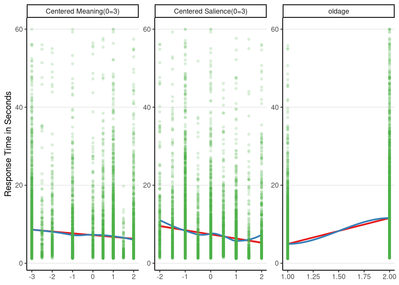
Residual Plots
# Get OLS residuals
m3_resid <- broom.mixed::augment(m3_rs) %>%
    mutate(.ols_resid = `log(rt_sec)` - .fixed)
# OLS residuals against predictted
ggplot(m3_resid, aes(x = .fixed, y = .ols_resid)) +
    geom_point(size = 0.7, alpha = 0.5) +
    geom_smooth(se = FALSE)
># `geom_smooth()` using method = 'gam' and formula = 'y ~ s(x, bs = "cs")'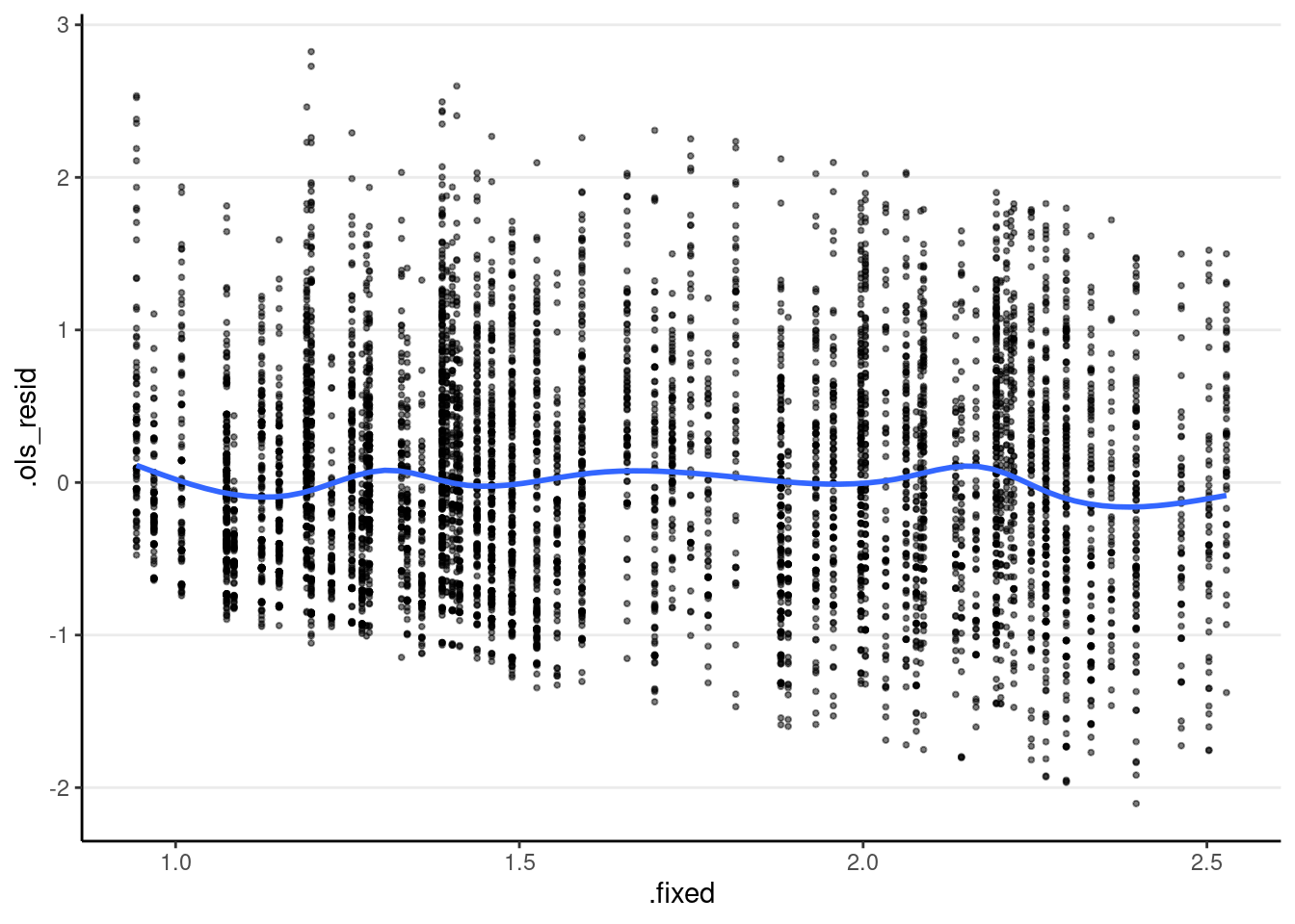
You can see an angled bound in the bottom left of the graph, which is due to the outcome being non-negative. You should plot the residuals against other predictors as well.