Week 3 (R): Random Intercept

Load Packages and Import Data

You can use the message = FALSE option to suppress the package loading messages.

# To install a package, run the following ONCE (and only once on your computer)
# install.packages("psych")
library(here)  # makes reading data more consistent
library(tidyverse)  # for data manipulation and plotting
library(haven)  # for importing SPSS/SAS/Stata data
library(lme4)  # for multilevel analysis
library(brms)  # for Bayesian multilevel analysis
library(lattice)  # for dotplot (working with lme4)
library(sjPlot)  # for plotting effects
library(MuMIn)  # for computing r-squared
library(r2mlm)  # for computing r-squared
library(modelsummary)  # for making tables

In R, there are many packages for multilevel modeling; two of the most common ones are the lme4 package and the nlme package. In this note, I will show how to run different basic multilevel models using the lme4 package, which is newer. However, some models, like unstructured covariance structure, will need the nlme package or other packages (like the brms package with Bayesian estimation).

Import Data

First, download the data from https://github.com/marklhc/marklai-pages/raw/master/data_files/hsball.sav. We’ll import the data in .sav format using the read_sav() function from the haven package.

# Read in the data (pay attention to the directory)
hsball <- read_sav(here("data_files", "hsball.sav"))
hsball # print the data

ABCDEFGHIJ0123456789

id <chr>	female <dbl>	ses <dbl>	mathach <dbl>	size <dbl>	pracad <dbl>
1224	1	-1.528	5.876	842	0.35
1224	1	-0.588	19.708	842	0.35
1224	0	-0.528	20.349	842	0.35
1224	0	-0.668	8.781	842	0.35
1224	0	-0.158	17.898	842	0.35
1224	0	0.022	4.583	842	0.35
1224	1	-0.618	-2.832	842	0.35
1224	0	-0.998	0.523	842	0.35
1224	1	-0.888	1.527	842	0.35
1224	0	-0.458	21.521	842	0.35

Run the Random Intercept Model

Model equations

Lv-1: ${mathach}_{i j} = β_{0 j} + e_{i j}$ where $β_{0 j}$ is the population mean math achievement of the $j$ th school, and $e_{i j}$ is the level-1 random error term for the $i$ th individual of the $j$ th school.

Lv-2: $β_{0 j} = γ_{00} + u_{0 j}$ where $γ_{00}$ is the grand mean, and $u_{0 j}$ is the deviation of the mean of the $j$ th school from the grand mean.

Running the model in R

The lme4 package requires input in the format of

outcome ~ fixed + (random | cluster ID)

For our data, the combined equation is ${mathach}_{i j} = γ_{00} + u_{0 j} + e_{i j},$ which we can explicitly write ${mathach}_{i j} = γ_{00} (1) + u_{0 j} (1) + e_{i j} .$ With that, we can see

outcome = mathach,
fixed = 1,
random = 1, and
cluster ID = id.

Thus the following syntax:

About brms: The brms package is a very powerful package that relies on Bayesian estimation, which we will discuss later in the class. I want to start introducing it because, moving forward, there are models that are difficult or impossible to estimate with lme4. If you cannot get brms to work, you may need to follow the instruction, which is different depending on your operating system, at https://github.com/stan-dev/rstan/wiki/RStan-Getting-Started to configure C++ Toolchain.

# outcome = mathach
# fixed = gamma_{00} * 1
# random = u_{0j} * 1, with j indexing school id
ran_int <- lmer(mathach ~ 1 + (1 | id), data = hsball)
# Summarize results
summary(ran_int)

Linear mixed model fit by REML ['lmerMod']
Formula: mathach ~ 1 + (1 | id)
   Data: hsball

REML criterion at convergence: 47116.8

Scaled residuals: 
    Min      1Q  Median      3Q     Max 
-3.0631 -0.7539  0.0267  0.7606  2.7426 

Random effects:
 Groups   Name        Variance Std.Dev.
 id       (Intercept)  8.614   2.935   
 Residual             39.148   6.257   
Number of obs: 7185, groups:  id, 160

Fixed effects:
            Estimate Std. Error t value
(Intercept)  12.6370     0.2444   51.71

# outcome = mathach
# fixed = gamma_{00} * 1
# random = u_{0j} * 1, with j indexing school id
ran_int_brm <- brm(mathach ~ 1 + (1 | id), data = hsball,
                   # cache results as brms takes a long time to run
                   file = "brms_cached_ran_int")
# Summarize results
summary(ran_int_brm)

 Family: gaussian 
  Links: mu = identity; sigma = identity 
Formula: mathach ~ 1 + (1 | id) 
   Data: hsball (Number of observations: 7185) 
  Draws: 4 chains, each with iter = 2000; warmup = 1000; thin = 1;
         total post-warmup draws = 4000

Group-Level Effects: 
~id (Number of levels: 160) 
              Estimate Est.Error l-95% CI u-95% CI Rhat Bulk_ESS Tail_ESS
sd(Intercept)     2.95      0.18     2.62     3.32 1.00     1153     2213

Population-Level Effects: 
          Estimate Est.Error l-95% CI u-95% CI Rhat Bulk_ESS Tail_ESS
Intercept    12.63      0.26    12.11    13.12 1.01      489      805

Family Specific Parameters: 
      Estimate Est.Error l-95% CI u-95% CI Rhat Bulk_ESS Tail_ESS
sigma     6.26      0.05     6.15     6.36 1.00     8936     2831

Draws were sampled using sampling(NUTS). For each parameter, Bulk_ESS
and Tail_ESS are effective sample size measures, and Rhat is the potential
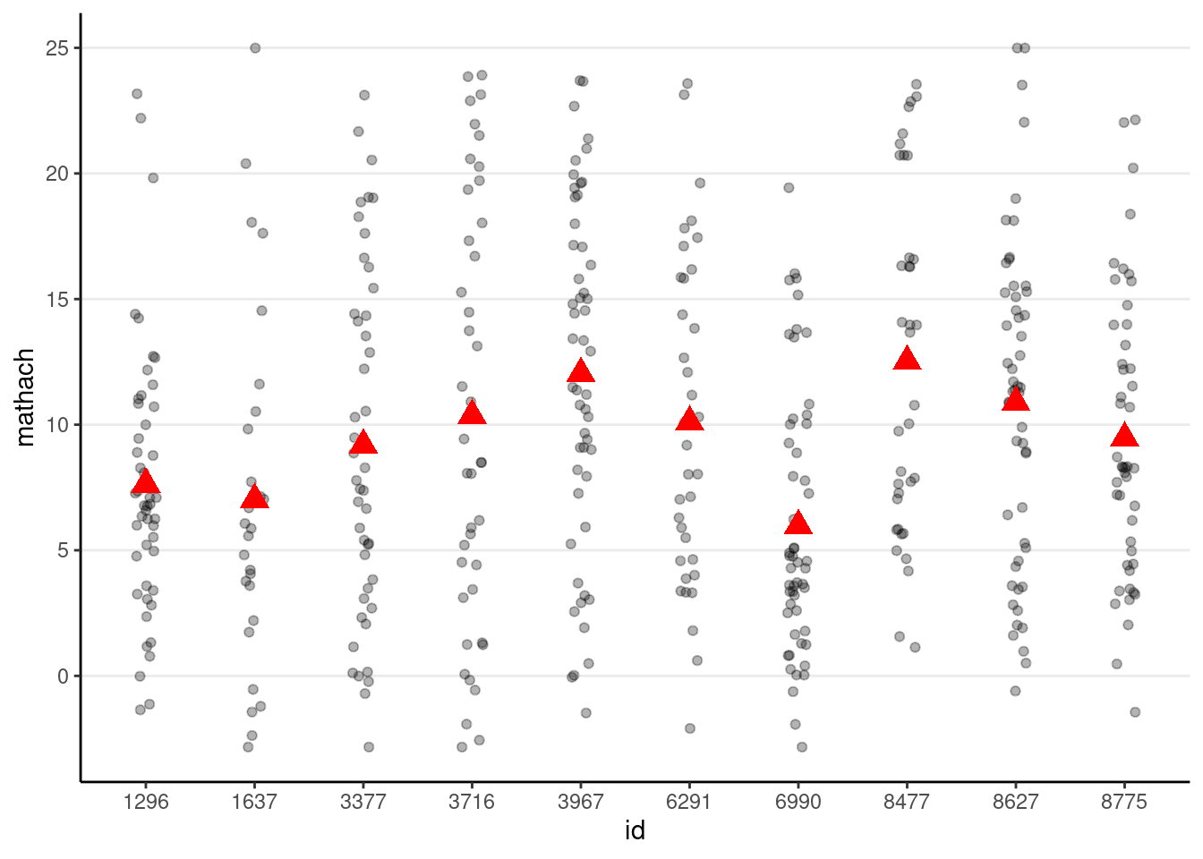
scale reduction factor on split chains (at convergence, Rhat = 1).

Showing the variations across (a subset of) schools

# Randomly select 10 school ids
set.seed(1330) # setting the seed for reproducibility
random_ids <- sample(unique(hsball$id), size = 10)
(p_subset <- hsball %>%
    filter(id %in% random_ids) %>% # select only 10 schools
    ggplot(aes(x = id, y = mathach)) +
    geom_jitter(height = 0, width = 0.1, alpha = 0.3) +
    # Add school means
    stat_summary(
        fun = "mean", geom = "point", col = "red",
        shape = 17, # use triangles
        size = 4 # make them larger
    )
)

Simulating data based on the random intercept model

$Y_{i j} = γ_{00} + u_{0 j} + e_{i j},$

gamma00 <- 12.6370
tau0 <- 2.935
sigma <- 6.257
num_students <- nrow(hsball)
num_schools <- length(unique(hsball$id))
# Simulate with only gamma00 (i.e., tau0 = 0 and sigma = 0)
simulated_data1 <- tibble(
    id = hsball$id,
    mathach = gamma00
)
# Show data with no variation
# The `%+%` operator is used to substitute with a different data set
p_subset %+%
    (simulated_data1 %>%
        filter(id %in% random_ids))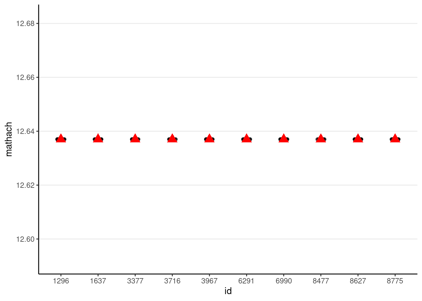

# Simulate with gamma00 + e_ij (i.e., tau0 = 0)
simulated_data2 <- tibble(
    id = hsball$id,
    mathach = gamma00 + rnorm(num_students, sd = sigma)
)
# Show data with no school-level variation
p_subset %+%
    (simulated_data2 %>%
        filter(id %in% random_ids))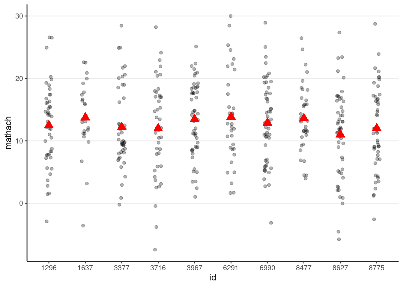

# Simulate with gamma00 + u_0j + e_ij
# First, obtain group indices that start from 1 to 160
group_idx <- group_by(hsball, id) %>% group_indices()
# Then simulate 160 u0j
u0j <- rnorm(num_schools, sd = tau0)
simulated_data3 <- tibble(
    id = hsball$id,
    mathach = gamma00 +
        u0j[group_idx] + # expand the u0j's from 160 to 7185
        rnorm(num_students, sd = sigma)
)
# Show data with both school and student variations
p_subset %+%
    (simulated_data3 %>%
        filter(id %in% random_ids))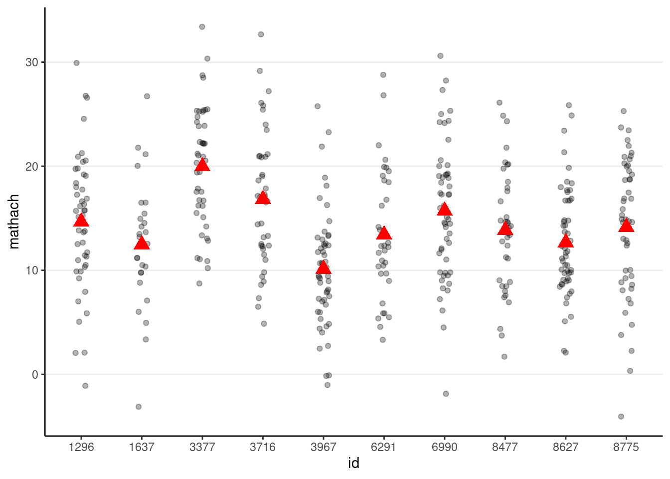

The handy simulate() function can also be used to simulate the data

simulated_math <- simulate(ran_int, nsim = 1)
simulated_data4 <- tibble(
    id = hsball$id,
    mathach = simulated_math$sim_1
)
p_subset %+%
    (simulated_data4 %>%
        filter(id %in% random_ids))

Plotting the random effects (i.e., $u_{0 j}$ )

You can easily plot the estimated school means (also called BLUP, best linear unbiased predictor, or the empirical Bayes (EB) estimates, which are different from the mean of the sample observations for a particular school) using the lattice package:

dotplot(ranef(ran_int, condVar = TRUE))

$id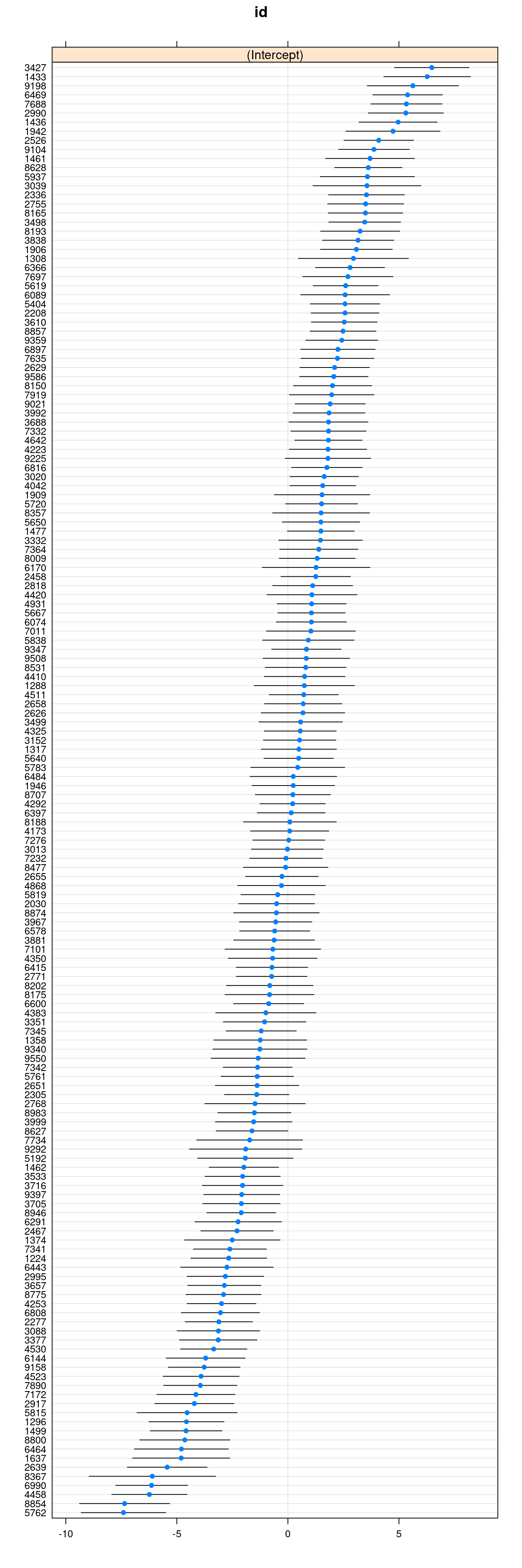

Or with sjPlot::plot_model()

plot_model(ran_int, type = "re")

Warning in checkMatrixPackageVersion(): Package version inconsistency detected.
TMB was built with Matrix version 1.5.1
Current Matrix version is 1.5.3
Please re-install 'TMB' from source using install.packages('TMB', type = 'source') or ask CRAN for a binary version of 'TMB' matching CRAN's 'Matrix' package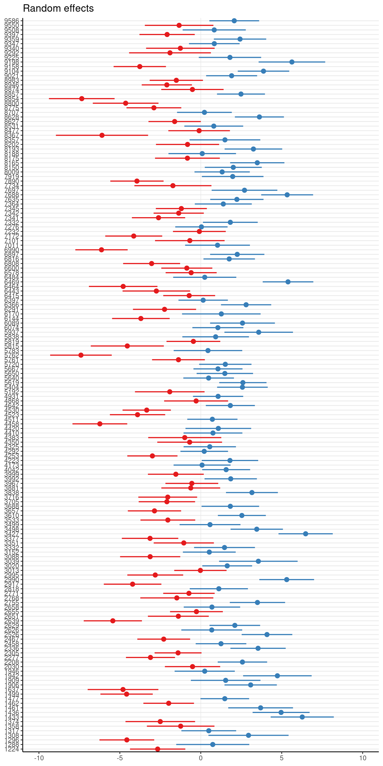

Here’s a plot showing the sample school means (with no borrowing of information) vs. the EB means (borrowing information).

# Compute raw school means and EB means
hsball %>%
    group_by(id) %>%
    # Raw means
    summarise(mathach_raw_means = mean(mathach)) %>%
    arrange(mathach_raw_means) %>% # sort by the means
    # EB means (the "." means using the current data)
    mutate(
        mathach_eb_means = predict(ran_int, .),
        index = row_number() # add row number as index for plotting
    ) %>%
    ggplot(aes(x = index, y = mathach_raw_means)) +
    geom_point(aes(col = "Raw")) +
    # Add EB means
    geom_point(aes(y = mathach_eb_means, col = "EB"), shape = 1) +
    geom_segment(aes(
        x = index, xend = index,
        y = mathach_eb_means, yend = mathach_raw_means,
        col = "EB"
    )) +
    labs(y = "School mean achievement", col = "")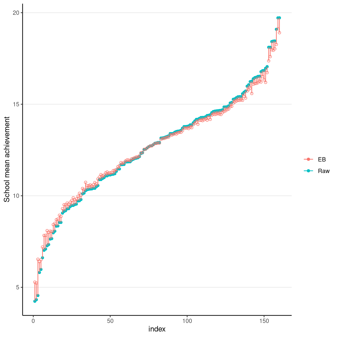

Intraclass correlations

variance_components <- as.data.frame(VarCorr(ran_int))
between_var <- variance_components$vcov[1]
within_var <- variance_components$vcov[2]
(icc <- between_var / (between_var + within_var))

[1] 0.1803518

# 95% confidence intervals (require installing the bootmlm package)
# if (!require("remotes")) {
#   install.packages("remotes")
# }
# remotes::install_github("marklhc/bootmlm")
bootmlm:::prof_ci_icc(ran_int)

    2.5 %    97.5 % 
0.1471784 0.2210131

Adding Lv-2 Predictors

We have one predictor, meanses, in the fixed part.

hsball %>%
    ggplot(aes(x = meanses, y = mathach, col = id)) +
    geom_point(alpha = 0.5, size = 0.5) +
    guides(col = "none")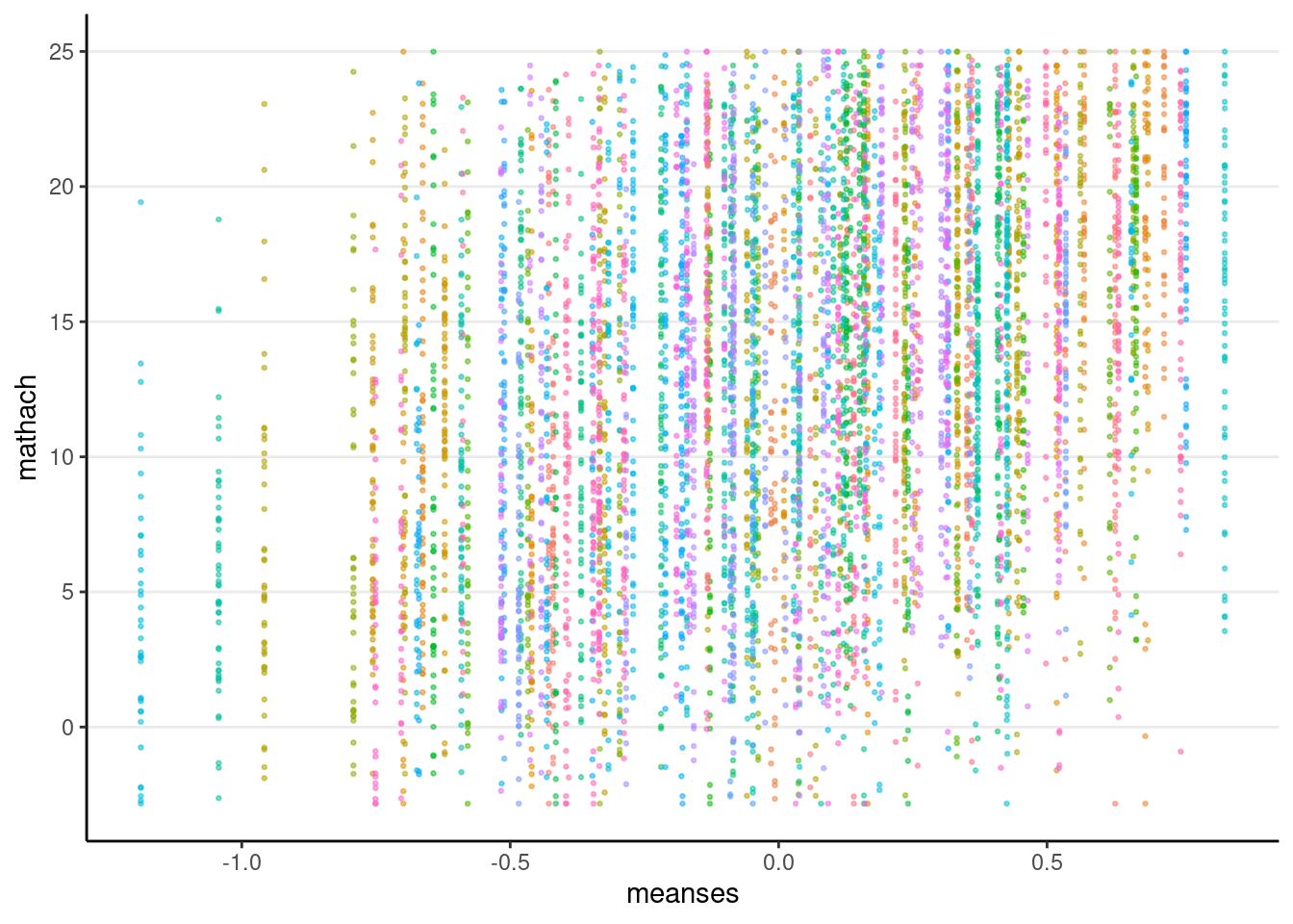

Model Equation

Lv-1:

${mathach}_{i j} = β_{0 j} + e_{i j}$

Lv-2:

$β_{0 j} = γ_{00} + γ_{01} {meanses}_{j} + u_{0 j}$ where $γ_{00}$ is the grand intercept, $γ_{10}$ is the regression coefficient of meanses that represents the expected difference in school mean achievement between two schools with one unit difference in meanses, and $u_{0 j}$ is the deviation of the mean of the $j$ th school from the grand mean.

m_lv2 <- lmer(mathach ~ meanses + (1 | id), data = hsball)
summary(m_lv2)

Linear mixed model fit by REML ['lmerMod']
Formula: mathach ~ meanses + (1 | id)
   Data: hsball

REML criterion at convergence: 46961.3

Scaled residuals: 
     Min       1Q   Median       3Q      Max 
-3.13480 -0.75256  0.02409  0.76773  2.78501 

Random effects:
 Groups   Name        Variance Std.Dev.
 id       (Intercept)  2.639   1.624   
 Residual             39.157   6.258   
Number of obs: 7185, groups:  id, 160

Fixed effects:
            Estimate Std. Error t value
(Intercept)  12.6494     0.1493   84.74
meanses       5.8635     0.3615   16.22

Correlation of Fixed Effects:
        (Intr)
meanses -0.004

# Likelihood-based confidence intervals for fixed effects
# `parm = "beta_"` requests confidence intervals only for the fixed effects
confint(m_lv2, parm = "beta_")

Computing profile confidence intervals ...

                2.5 %    97.5 %
(Intercept) 12.356615 12.941707
meanses      5.155769  6.572415

m_lv2_brm <- brm(mathach ~ meanses + (1 | id), data = hsball,
                 # cache results as brms takes a long time to run
                 file = "brms_cached_m_lv2")
summary(m_lv2_brm)

 Family: gaussian 
  Links: mu = identity; sigma = identity 
Formula: mathach ~ meanses + (1 | id) 
   Data: hsball (Number of observations: 7185) 
  Draws: 4 chains, each with iter = 2000; warmup = 1000; thin = 1;
         total post-warmup draws = 4000

Group-Level Effects: 
~id (Number of levels: 160) 
              Estimate Est.Error l-95% CI u-95% CI Rhat Bulk_ESS Tail_ESS
sd(Intercept)     1.64      0.13     1.40     1.91 1.00     1485     2069

Population-Level Effects: 
          Estimate Est.Error l-95% CI u-95% CI Rhat Bulk_ESS Tail_ESS
Intercept    12.65      0.15    12.37    12.94 1.00     1961     2566
meanses       5.86      0.37     5.16     6.57 1.00     2126     2836

Family Specific Parameters: 
      Estimate Est.Error l-95% CI u-95% CI Rhat Bulk_ESS Tail_ESS
sigma     6.26      0.05     6.16     6.36 1.00     9510     3281

Draws were sampled using sampling(NUTS). For each parameter, Bulk_ESS
and Tail_ESS are effective sample size measures, and Rhat is the potential
scale reduction factor on split chains (at convergence, Rhat = 1).

The 95% confidence intervals (CIs) above showed the uncertainty associated with the estimates. Also, as the 95% CI for meanses does not contain zero, there is evidence for the positive association of SES and mathach at the school level.

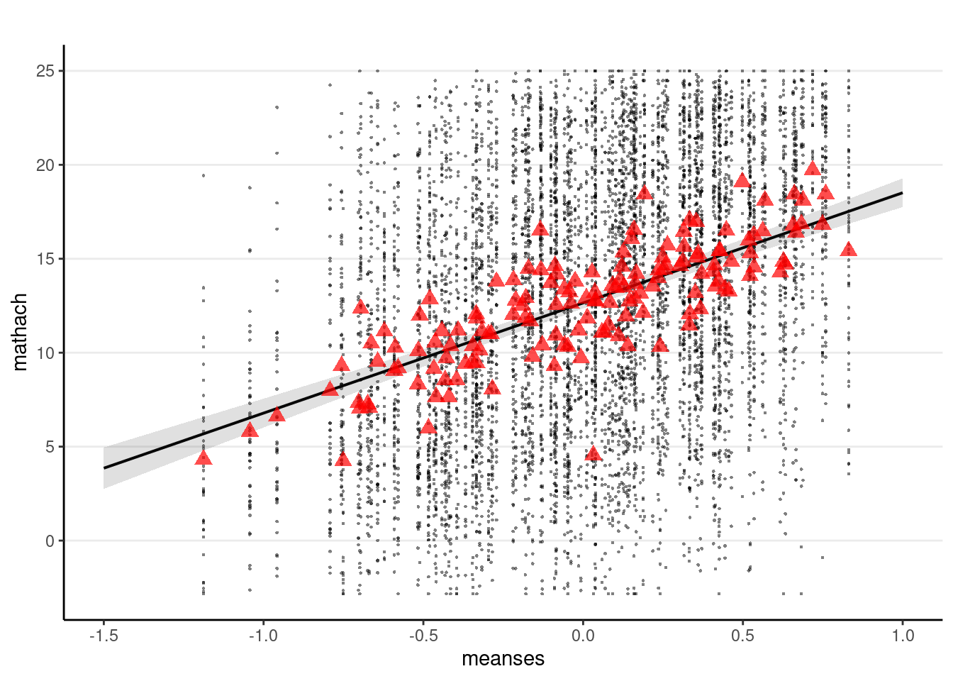
sjPlot::plot_model(m_lv2,
    type = "pred", terms = "meanses",
    show.data = TRUE, title = "",
    dot.size = 0.5
) +
    # Add the group means
    stat_summary(
        data = hsball, aes(x = meanses, y = mathach),
        fun = mean, geom = "point",
        col = "red",
        shape = 17,
        # use triangles
        size = 3,
        alpha = 0.7
    )

Proportion of variance predicted

We will use the $R^{2}$ statistic proposed by Nakagawa, Johnson & Schielzeth (2017) to obtain an $R^{2}$ statistic. There are multiple versions of $R^{2}$ in the literature, but personally, this $R^{2}$ avoids many of the problems in other variants and is most meaningful to interpret. Note that I only interpret the marginal $R^{2}$ .

# Generally, you should use the marginal R^2 (R2m) for the variance predicted by
# your predictors (`meanses` in this case).
MuMIn::r.squaredGLMM(m_lv2)

Warning: 'r.squaredGLMM' now calculates a revised statistic. See the help page.

           R2m       R2c
[1,] 0.1233346 0.1786815

An alternative, more comprehensive approach is by Rights & Sterba (2019, Psychological Methods, https://doi.org/10.1037/met0000184), with the r2mlm package

r2mlm::r2mlm(m_lv2)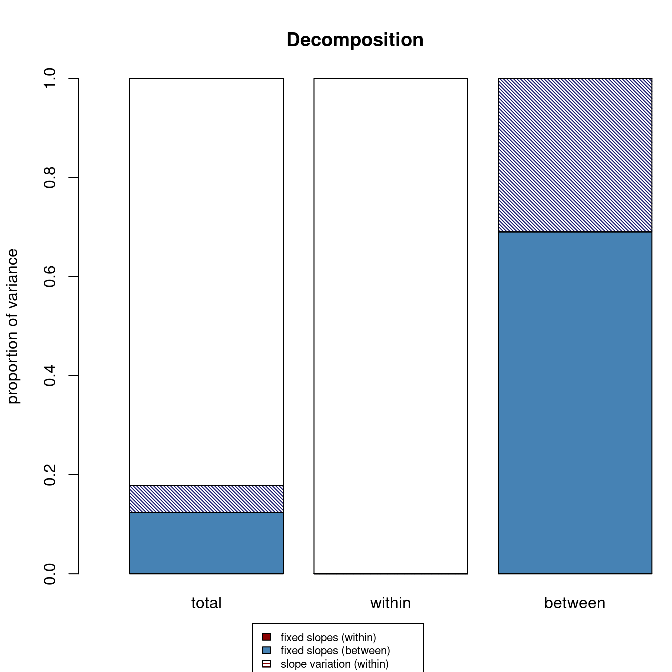

$Decompositions
                     total within   between
fixed, within   0.00000000      0        NA
fixed, between  0.12333464     NA 0.6902487
slope variation 0.00000000      0        NA
mean variation  0.05534682     NA 0.3097513
sigma2          0.82131854      1        NA

$R2s
         total within   between
f1  0.00000000      0        NA
f2  0.12333464     NA 0.6902487
v   0.00000000      0        NA
m   0.05534682     NA 0.3097513
f   0.12333464     NA        NA
fv  0.12333464      0        NA
fvm 0.17868146     NA        NA

Note the fixed, between number in the total column is the same as the one from MuMIn::r.squaredGLMM(). Including school means of SES in the model accounted for about 12% of the total variance of math achievement.

Comparing to OLS regression

Notice that the standard error with regression is only half of that with MLM.

m_lm <- lm(mathach ~ meanses, data = hsball)
msummary(list("MLM" = m_lv2,
              "Linear regression" = m_lm))

	MLM	Linear regression
(Intercept)	12.649	12.713
	(0.149)	(0.076)
meanses	5.864	5.717
	(0.361)	(0.184)
SD (Intercept id)	1.624
SD (Observations)	6.258
Num.Obs.	7185	7185
R2		0.118
R2 Adj.		0.118
R2 Marg.	0.123
R2 Cond.	0.179
AIC	46969.3	47202.4
BIC	46996.8	47223.0
ICC	0.06
Log.Lik.		−23598.190
F		962.329
RMSE	6.21	6.46