# To install a package, run the following ONCE (and only once on your computer)
# install.packages("psych")
library(here)  # makes reading data more consistent
library(tidyverse)  # for data manipulation and plotting
library(haven)  # for importing SPSS/SAS/Stata data
library(lme4)  # for multilevel analysis
library(brms)  # for Bayesian estimation
library(MuMIn)  # for computing r-squared
library(modelsummary)  # for making tables
library(sjPlot) # for plotting effectsWeek 5 (R): Testing
\[ \newcommand{\bv}[1]{\boldsymbol{\mathbf{#1}}} \]
Load Packages and Import Data
# Read in the data (pay attention to the directory)
hsball <- read_sav(here("data_files", "hsball.sav"))
To demonstrate differences in smaller samples, we will use a subset of 16 schools.
# Randomly select 16 school ids
set.seed(840)  # use the same seed so that the same 16 schools are selected
random_ids <- sample(unique(hsball$id), size = 16)
hsbsub <- hsball %>%
    filter(id %in% random_ids)
Log-Likelihood Function \(\ell\)
Example: \(\ell(\gamma_{01})\)
We’ll use the model with meanses as the predictor on the original data set (hsball), and use R to write the log-likelihood function for \(\gamma_{01}\)
# Extract V from the model
V_m_lv2 <- (crossprod(getME(m_lv2, "A")) + Matrix::Diagonal(7185)) *
    sigma(m_lv2)^2
# Log-likelihood function with respect to gamma01
llfun <- function(gamma01,
                  gamma00 = fixef(m_lv2)[1],
                  y = m_lv2@resp$y,
                  X = cbind(1, m_lv2@frame$meanses),
                  V = V_m_lv2) {
    gamma <- c(gamma00, gamma01)
    y_minus_Xgamma <- y - X %*% gamma
    as.numeric(
        - crossprod(y_minus_Xgamma, solve(V, y_minus_Xgamma)) / 2
    )
}
# Vectorize
llfun <- Vectorize(llfun)
# Plot
ggplot(tibble(gamma01 = c(5, 7)), aes(x = gamma01)) +
    stat_function(fun = llfun) +
    labs(x = expression(gamma[0][1]), y = "log(Likelihood)")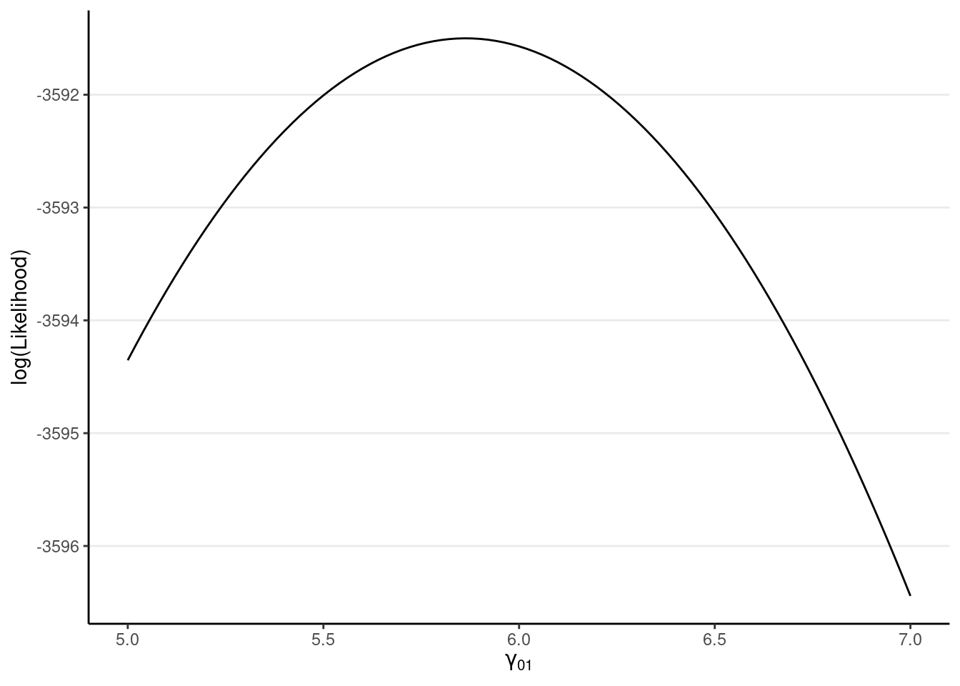
Standard Errors
Without going into too much detail, the sampling variance (i.e., the squared value of the standard error) can be approximated by the curvature of the likelihood function around the neighborhood of the maximum likelihood estimate. This is however only an approximation, and is generally an underestimate unless the sample size is large. Therefore, the estimated standard errors are usually called the asymptotic standard errors, meaning they converge to the correct values when the sample size is large.
In R:
# Asympotitc standard error (ASE) from lme4
vcov(m_lv2)
># 2 x 2 Matrix of class "dpoMatrix"
># (Intercept) meanses
># (Intercept) 0.0222845612 -0.0002358047
># meanses -0.0002358047 0.1306518973The standard errors are the square root values of the diagonal elements.
sqrt(diag(vcov(m_lv2))) # check with the standard errors in the model># (Intercept) meanses
># 0.1492801 0.3614580ML vs REML
We’ll use the cross-level interaction model on the subset
# Cluster-mean centering
hsbsub <- hsbsub %>%
    group_by(id) %>%   # operate within schools
    mutate(ses_cm = mean(ses),   # create cluster means (the same as `meanses`)
           ses_cmc = ses - ses_cm) %>%   # cluster-mean centered
    ungroup()  # exit the "editing within groups" mode
# Default is REML
crlv_int <- lmer(mathach ~ meanses + sector * ses_cmc + (ses_cmc | id),
                 data = hsbsub)
># boundary (singular) fit: see help('isSingular')# Use REML = FALSE for ML
crlv_int_ml <- lmer(mathach ~ meanses + sector * ses_cmc + (ses_cmc | id),
data = hsbsub, REML = FALSE)># boundary (singular) fit: see help('isSingular')# Alternatively, you can use refitML()
# refitML(crlv_int_ml)
# Compare the models
msummary(list("REML" = crlv_int,
"ML" = crlv_int_ml))| REML | ML | |
|---|---|---|
| (Intercept) | 11.728 | 11.728 |
| (0.670) | (0.605) | |
| meanses | 6.633 | 6.492 |
| (1.139) | (1.035) | |
| sector | 1.890 | 1.901 |
| (0.903) | (0.815) | |
| ses_cmc | 2.860 | 2.862 |
| (0.464) | (0.459) | |
| sector × ses_cmc | −0.885 | −0.888 |
| (0.661) | (0.655) | |
| SD (Intercept id) | 1.520 | 1.317 |
| SD (ses_cmc id) | 0.354 | 0.311 |
| Cor (Intercept~ses_cmc id) | 1.000 | 1.000 |
| SD (Observations) | 5.698 | 5.689 |
| Num.Obs. | 686 | 686 |
| R2 Marg. | 0.248 | 0.247 |
| R2 Cond. | 0.299 | 0.286 |
| AIC | 4365.1 | 4365.4 |
| BIC | 4405.9 | 4406.2 |
| ICC | 0.07 | 0.05 |
| RMSE | 5.64 | 5.64 |
Notice that the standard errors are generally larger for REML than for ML, and it’s generally more accurate with REML in small samples. Also the \(\tau^2\) estimates (i.e., labelled sd__(Intercept) for \(\tau^2_0\) and sd__ses_cmc for \(\tau^2_1\)) are larger (and more accurately estimated) for REML.
To see more details on how lme4 iteratively tries to arrive at the REML/ML estimates, try
crlv_int2 <- lmer(mathach ~ meanses + sector * ses_cmc + (ses_cmc | id),
                  data = hsbsub, verbose = 1)
># iteration: 1
># f(x) = 4396.943300
># iteration: 2
># f(x) = 4410.471845
># iteration: 3
># f(x) = 4398.478905
># iteration: 4
># f(x) = 4411.654851
># iteration: 5
># f(x) = 4377.931282
># iteration: 6
># f(x) = 4399.307646
># iteration: 7
># f(x) = 4371.367019
># iteration: 8
># f(x) = 4347.537222
># iteration: 9
># f(x) = 4367.879802
># iteration: 10
># f(x) = 4350.984197
># iteration: 11
># f(x) = 4351.658449
># iteration: 12
># f(x) = 4349.986861
># iteration: 13
># f(x) = 4347.709342
># iteration: 14
># f(x) = 4347.884914
># iteration: 15
># f(x) = 4347.701287
># iteration: 16
># f(x) = 4347.194148
># iteration: 17
># f(x) = 4347.172072
># iteration: 18
># f(x) = 4347.140652
># iteration: 19
># f(x) = 4347.137326
># iteration: 20
># f(x) = 4347.127020
># iteration: 21
># f(x) = 4347.128477
># iteration: 22
># f(x) = 4347.143600
># iteration: 23
># f(x) = 4347.125497
># iteration: 24
># f(x) = 4347.125875
># iteration: 25
># f(x) = 4347.125844
># iteration: 26
># f(x) = 4347.125305
># iteration: 27
># f(x) = 4347.125138
># iteration: 28
># f(x) = 4347.125098
># iteration: 29
># f(x) = 4347.125226
># iteration: 30
># f(x) = 4347.125068
># iteration: 31
># f(x) = 4347.125119
># iteration: 32
># f(x) = 4347.125062
># iteration: 33
># f(x) = 4347.125065
># iteration: 34
># f(x) = 4347.125063
># iteration: 35
># f(x) = 4347.125066
># iteration: 36
># f(x) = 4347.125059
># iteration: 37
># f(x) = 4347.125056
># iteration: 38
># f(x) = 4347.125056># boundary (singular) fit: see help('isSingular')The numbers shown above are the deviance, that is, -2 \(\times\) log-likelihood. Because probabilities (as well as likelihood) are less than or equal to 1, the log will be less than or equal to 0, meaning that the log-likelihood values are generally negative. Multiplying it by -2 results in deviance, which is positive and is a bit easier to work with (and the factor 2 is related to converting a normal distribution to a \(\chi^2\) distribution).
Testing Fixed Effects
An easy way To test the null that a predictor has a non-zero fixed-effect coefficient (given other predictors in the model) is to use the likelihood-based 95% CI (also called the profile-likelihood CI, as discussed in your text):
# Use parm = "beta_" for only fixed effects
confint(crlv_int, parm = "beta_")
># Computing profile confidence intervals ...># 2.5 % 97.5 %
># (Intercept) 10.4692542 12.9863640
># meanses 4.0885277 8.9516323
># sector 0.1875109 3.5912615
># ses_cmc 1.9257690 3.7740789
># sector:ses_cmc -2.1748867 0.4629693If 0 is not in the 95% CI, the null is rejected at .05 significance level. This is equivalent to the likelihood ratio test, which can be obtained by comparing the model without one of the coefficients (e.g., the cross-level interaction):
model_no_crlv <- lmer(mathach ~ meanses + sector + ses_cmc + (ses_cmc | id),
                      data = hsbsub)
># boundary (singular) fit: see help('isSingular')# Note: lme4 will refit the model to use ML when performing LRT
anova(crlv_int, model_no_crlv)># refitting model(s) with ML (instead of REML)Or with the drop1() function and adding the formula:
# Note: lme4 will refit the model to use ML when performing LRT for fixed
# effects
drop1(crlv_int, ~ meanses + sector * ses_cmc, test = "Chisq")
># boundary (singular) fit: see help('isSingular')
># boundary (singular) fit: see help('isSingular')
># boundary (singular) fit: see help('isSingular')Small-Sample Correction: Kenward-Roger Approximation of Degrees of Freedom
In small sample situations (with < 50 clusters), the Kenward-Roger (KR) approximation of degrees of freedom will give more accurate standard errors and tests. To do this in R, you should load the lmerTest package before running the model. Since I’ve already run the model, I will load the package and convert the results using the as_lmerModLmerTest() function:
library(lmerTest)
crlv_int_test <- as_lmerModLmerTest(crlv_int)
# Try anova()
anova(crlv_int_test, ddf = "Kenward-Roger")
# Summary will print t test results
summary(crlv_int_test, ddf = "Kenward-Roger")># Linear mixed model fit by REML. t-tests use Kenward-Roger's method [
># lmerModLmerTest]
># Formula: mathach ~ meanses + sector * ses_cmc + (ses_cmc | id)
># Data: hsbsub
>#
># REML criterion at convergence: 4347.1
>#
># Scaled residuals:
># Min 1Q Median 3Q Max
># -3.11430 -0.75641 0.02989 0.72275 2.25163
>#
># Random effects:
># Groups Name Variance Std.Dev. Corr
># id (Intercept) 2.3097 1.5198
># ses_cmc 0.1255 0.3542 1.00
># Residual 32.4620 5.6975
># Number of obs: 686, groups: id, 16
>#
># Fixed effects:
># Estimate Std. Error df t value Pr(>|t|)
># (Intercept) 11.7282 0.6704 13.2107 17.493 1.6e-10 ***
># meanses 6.6327 1.2198 13.0241 5.438 0.000113 ***
># sector 1.8900 0.9049 13.2258 2.089 0.056618 .
># ses_cmc 2.8601 0.4805 8.6559 5.953 0.000250 ***
># sector:ses_cmc -0.8848 0.6788 11.7341 -1.303 0.217412
># ---
># Signif. codes: 0 '***' 0.001 '**' 0.01 '*' 0.05 '.' 0.1 ' ' 1
>#
># Correlation of Fixed Effects:
># (Intr) meanss sector ss_cmc
># meanses -0.021
># sector -0.738 -0.176
># ses_cmc 0.253 -0.020 -0.184
># sctr:ss_cmc -0.178 0.007 0.232 -0.701
># optimizer (nloptwrap) convergence code: 0 (OK)
># boundary (singular) fit: see help('isSingular')# Table (need to specify the `ci_method` argument)
msummary(list(`REML-KR` = crlv_int),
estimate = "{estimate} [{conf.low}, {conf.high}]",
statistic = NULL,
ci_method = "Kenward")| REML-KR | |
|---|---|
| (Intercept) | 11.728 [10.282, 13.174] |
| meanses | 6.633 [3.998, 9.267] |
| sector | 1.890 [−0.062, 3.842] |
| ses_cmc | 2.860 [1.767, 3.954] |
| sector × ses_cmc | −0.885 [−2.368, 0.598] |
| SD (Intercept id) | 1.520 |
| SD (ses_cmc id) | 0.354 |
| Cor (Intercept~ses_cmc id) | 1.000 |
| SD (Observations) | 5.698 |
| Num.Obs. | 686 |
| R2 Marg. | 0.248 |
| R2 Cond. | 0.299 |
| AIC | 4365.1 |
| BIC | 4405.9 |
| ICC | 0.07 |
| RMSE | 5.64 |
You can see now sector was actually not significant (although it is part of an interaction, so the coefficient reflects a conditional effect). Note KR requires using REML.
If you’re interested in knowing more, KR is based on an \(F\) test instead of a \(\chi^2\) test for LRT. When the denominator degrees of freedom for \(F\) is large, which happens in large samples (with many clusters), the \(F\) distribution converges to a \(\chi^2\) distribution, so there is no need to know what exactly the degrees of freedom are. However, in small samples, these two look different, and to get more accurate \(p\) values, one needs to have a good estimate of the denominator degrees of freedom, but it’s not straightforward with MLM, especially with unbalanced data (i.e., clusters having different sizes). There are several methods to approximate the degrees of freedom; KR is generally found to perform the best.
Testing Random Slopes
To test the null hypothesis that the random slope variance, \(\tau^2_1\), is zero, one can again rely on the LRT. However, because \(\tau^2_1\) is non-negative (i.e., zero or positive), using the regular LRT will lead to an overly conservative test, meaning that power is too small. Technically, as pointed out in your text, under the null, the sampling distribution of the LRT will follow approximately a mixture \(\chi^2\) distribution. There are several ways to improve the test, but as shown in LaHuis and Ferguson (2009, https://doi.org/10.1177/1094428107308984), a simple way is to divide the \(p\) value you obtain from software by 2 so that it resembles a one-tailed test.
ran_slp <- lmer(mathach ~ meanses + ses_cmc + (ses_cmc | id), data = hsbsub)
# Compare to the model without random slopes
m_bw <- lmer(mathach ~ meanses + ses_cmc + (1 | id), data = hsbsub)
# Compute the difference in deviance (4356.769 - 4356.754)
REMLcrit(m_bw) - REMLcrit(ran_slp)
># [1] 0.01432169# Find the p value from a chi-squared distribution
pchisq(REMLcrit(m_bw) - REMLcrit(ran_slp), df = 2, lower.tail = FALSE)># [1] 0.9928647# Need to divide the p by 2 for a one-tailed testSo the \(p\) value in our example for testing the random slope variance was 0.5, which suggested that for the subsample, there was insufficient evidence that the slope between ses_cmc and mathach varied across schools.
You can also use ranova() to get the same results (again, the \(p\) values need to be divided by 2)
ranova(ran_slp)Bootstrap
The bootstrap is a simulation-based method to approximate the sampling distribution of parameter estimates. Indeed, you’ve already seen a version of it in previous weeks when we talk about simulation. In previous weeks, we generated data assuming that the sample model perfectly described the population, including the normality assumption. That simulation method is also called parametric bootstrap. Here we’ll use another version of the bootstrap, called the residual bootstrap, which does not assume normality for the population. You can check out Lai (2021).
To perform the bootstrap, you’ll need to supply functions that extract different parameter estimates or other quantities (e.g., effect sizes) from a fitted model. Below are some examples:
Fixed Effects
library(boot)
# If you have not installed bootmlm, you can uncomment the following line:
# remotes::install_github("marklhc/bootmlm")
library(bootmlm)
Note: Because running the bootstrap takes a long time, you can include the chunk option
cache = TRUEso that when knitting the file, it will not rerun the chunk unless the code has been changed.
# This takes a few minutes to run
boot_crlv_int <- bootstrap_mer(
    crlv_int,  # model
    # function for extracting information from model (fixef = fixed effect)
    fixef,
    nsim = 1999,  # number of bootstrap samples
    type = "residual"  # residual bootstrap
)
# Bootstrap CI for cross-level interaction (index = 5 for 5th coefficient)
# Note: type = "perc" extracts the percentile CI, one of the several
# possible CI options with the bootstrap
boot.ci(boot_crlv_int, index = 5, type = "perc")
># BOOTSTRAP CONFIDENCE INTERVAL CALCULATIONS
># Based on 1999 bootstrap replicates
>#
># CALL :
># boot.ci(boot.out = boot_crlv_int, type = "perc", index = 5)
>#
># Intervals :
># Level Percentile
># 95% (-2.1774, 0.4368 )
># Calculations and Intervals on Original ScaleVariance Components
Extracting variance components from lmer() results requires a bit more efforts.
ran_slp <- lmer(mathach ~ meanses + ses_cmc + (ses_cmc | id), data = hsbsub)
# Define function to extract variance components
get_vc <- function(object) {
    vc_df <- data.frame(VarCorr(object))
    vc_df[, "vcov"]
}
# Verfiy that the function extracts the right quantities
get_vc(ran_slp)
># [1] 3.04994425 0.04159963 0.08850399 32.55971461# This again takes a few minutes to run
boot_ran_slp <- bootstrap_mer(
ran_slp, # model
# function for extracting information from model (random effect variances)
get_vc,
nsim = 1999, # number of bootstrap samples
type = "residual" # residual bootstrap
)
# Bootstrap CI for random slope variance (index = 2)
boot.ci(boot_ran_slp, index = 2, type = "perc")># BOOTSTRAP CONFIDENCE INTERVAL CALCULATIONS
># Based on 1999 bootstrap replicates
>#
># CALL :
># boot.ci(boot.out = boot_ran_slp, type = "perc", index = 2)
>#
># Intervals :
># Level Percentile
># 95% ( 0.0004, 1.4213 )
># Calculations and Intervals on Original Scale\(R^2\)
# This again takes a few minutes
boot_r2 <- bootstrap_mer(crlv_int, MuMIn::r.squaredGLMM, nsim = 1999,
                         type = "residual")
boot.ci(boot_r2, index = 1, type = "perc")  # index = 1 for marginal R2
># BOOTSTRAP CONFIDENCE INTERVAL CALCULATIONS
># Based on 1999 bootstrap replicates
>#
># CALL :
># boot.ci(boot.out = boot_r2, type = "perc", index = 1)
>#
># Intervals :
># Level Percentile
># 95% ( 0.1672, 0.3436 )
># Calculations and Intervals on Original ScaleYou can check the bootstrap sampling distribution using
plot(boot_r2, index = 1)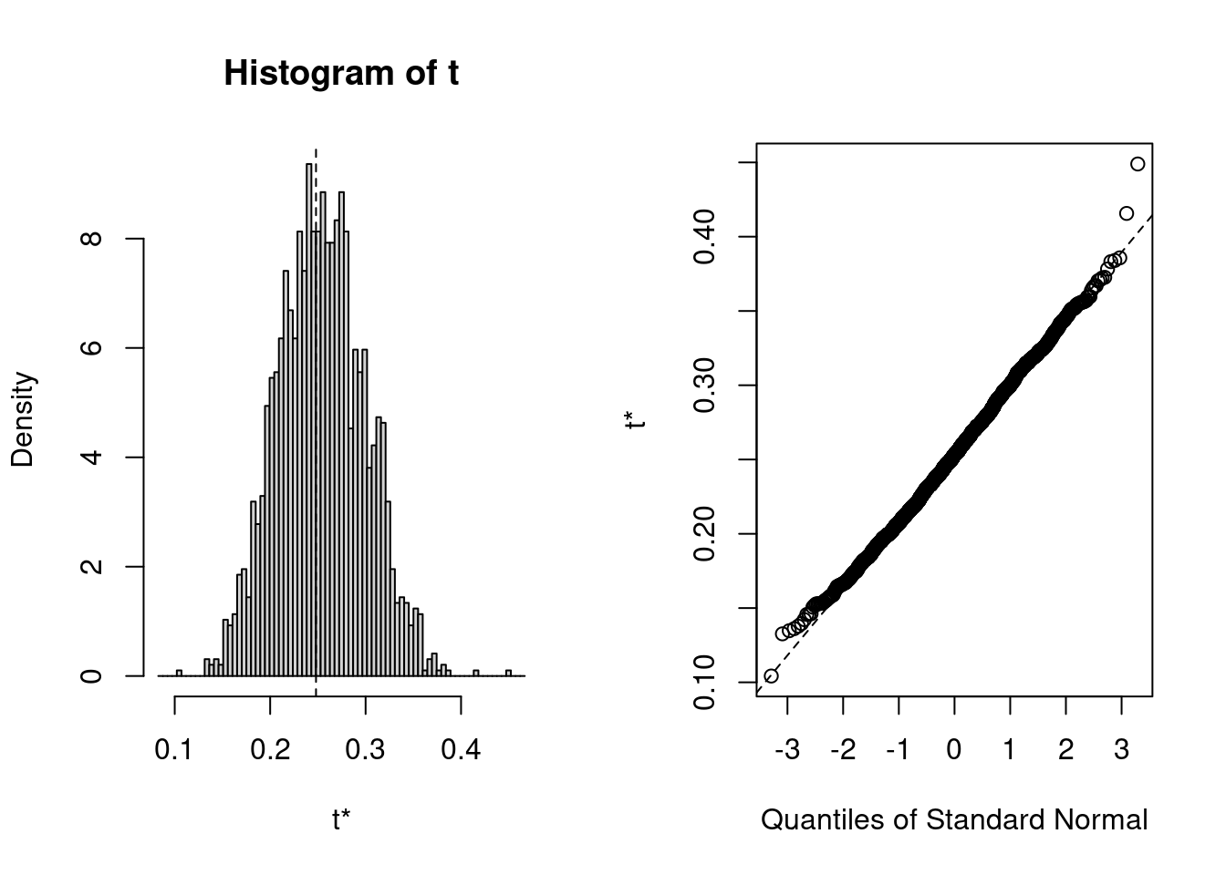
Bonus: Bias-corrected estimates
The bootstrap method is commonly used for obtaining standard errors and confidence intervals. You can get the bootstrap standard error:
boot_r2>#
># ORDINARY NONPARAMETRIC BOOTSTRAP
>#
>#
># Call:
># bootstrap_mer(x = crlv_int, FUN = MuMIn::r.squaredGLMM, nsim = 1999,
># type = "residual")
>#
>#
># Bootstrap Statistics :
># original bias std. error
># t1* 0.2480355 0.005799343 0.04522714
># t2* 0.2991689 0.005804885 0.04657592The above also showed the original estimate for the marginal \(R^2\) (in row 1), 0.2480355, and the estimated bias using the bootstrap, which suggested that the bias is slightly upward. Therefore, one can obtain the bias-corrected estimate by
\[\text{Bias-corrected estimate} = \text{Original estimate} - \text{Bias}\]
You can also use the following R code:
# Bias
mean(boot_r2$t[, 1]) - boot_r2$t0[1]  # the first index is marginal R^2; second is conditional R^2
># [1] 0.005799343# Bias-corrected estimate
2 * boot_r2$t0[1] - mean(boot_r2$t[, 1])># [1] 0.2422361Bayesian (Markov Chain Monte Carlo; MCMC) Estimation
Using brms
Basically, just change lmer() to brm().
crlv_int_brm <- brm(mathach ~ meanses + sector * ses_cmc + (ses_cmc | id),
                    data = hsbsub,
                    # cache results as brms takes a long time to run
                    file = "brms_cached_crlv_int")
This takes longer to run; however, the payoff is great, as
- Bayesian estimation generally has better small sample properties,
- it solves many of the convergence issues you will run into using
lme4, brmssupports many more complex models (see Table 1 of this paper; e.g., spatial and temporal correlations; zero-inflated and survival models; mediation; meta-analysis)brmsand Bayesian estimation are getting more and more popular in recent MLM literature
For more complex models, using brms may save you time troubleshooting why your model does not converge.
Here is a summary of the results
summary(crlv_int_brm)># Family: gaussian
># Links: mu = identity; sigma = identity
># Formula: mathach ~ meanses + sector * ses_cmc + (ses_cmc | id)
># Data: hsbsub (Number of observations: 686)
># Draws: 4 chains, each with iter = 2000; warmup = 1000; thin = 1;
># total post-warmup draws = 4000
>#
># Group-Level Effects:
># ~id (Number of levels: 16)
># Estimate Est.Error l-95% CI u-95% CI Rhat Bulk_ESS
># sd(Intercept) 1.70 0.49 0.95 2.81 1.00 1394
># sd(ses_cmc) 0.54 0.41 0.02 1.54 1.00 1771
># cor(Intercept,ses_cmc) 0.19 0.54 -0.88 0.96 1.00 3211
># Tail_ESS
># sd(Intercept) 2093
># sd(ses_cmc) 2121
># cor(Intercept,ses_cmc) 2348
>#
># Population-Level Effects:
># Estimate Est.Error l-95% CI u-95% CI Rhat Bulk_ESS Tail_ESS
># Intercept 11.76 0.73 10.27 13.20 1.00 1931 2460
># meanses 6.27 1.43 3.48 9.12 1.00 1354 1767
># sector 1.91 0.99 -0.03 3.89 1.00 1990 2348
># ses_cmc 2.85 0.51 1.81 3.84 1.00 2947 2401
># sector:ses_cmc -0.90 0.72 -2.26 0.59 1.00 3026 2180
>#
># Family Specific Parameters:
># Estimate Est.Error l-95% CI u-95% CI Rhat Bulk_ESS Tail_ESS
># sigma 5.71 0.16 5.42 6.03 1.00 7697 3131
>#
># Draws were sampled using sampling(NUTS). For each parameter, Bulk_ESS
># and Tail_ESS are effective sample size measures, and Rhat is the potential
># scale reduction factor on split chains (at convergence, Rhat = 1).The terms under “Group-Level Effects” are the random effect standard deviations (i.e., the \(\tau\)s). The terms under “Population-Level Effects” are the fixed effects (i.e., the \(\gamma\)s). Note that with Bayesian, you generally get standard errors for everything (in the column “Est.Error”).
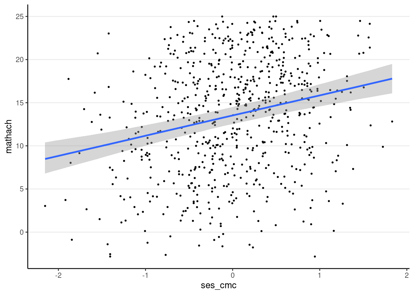
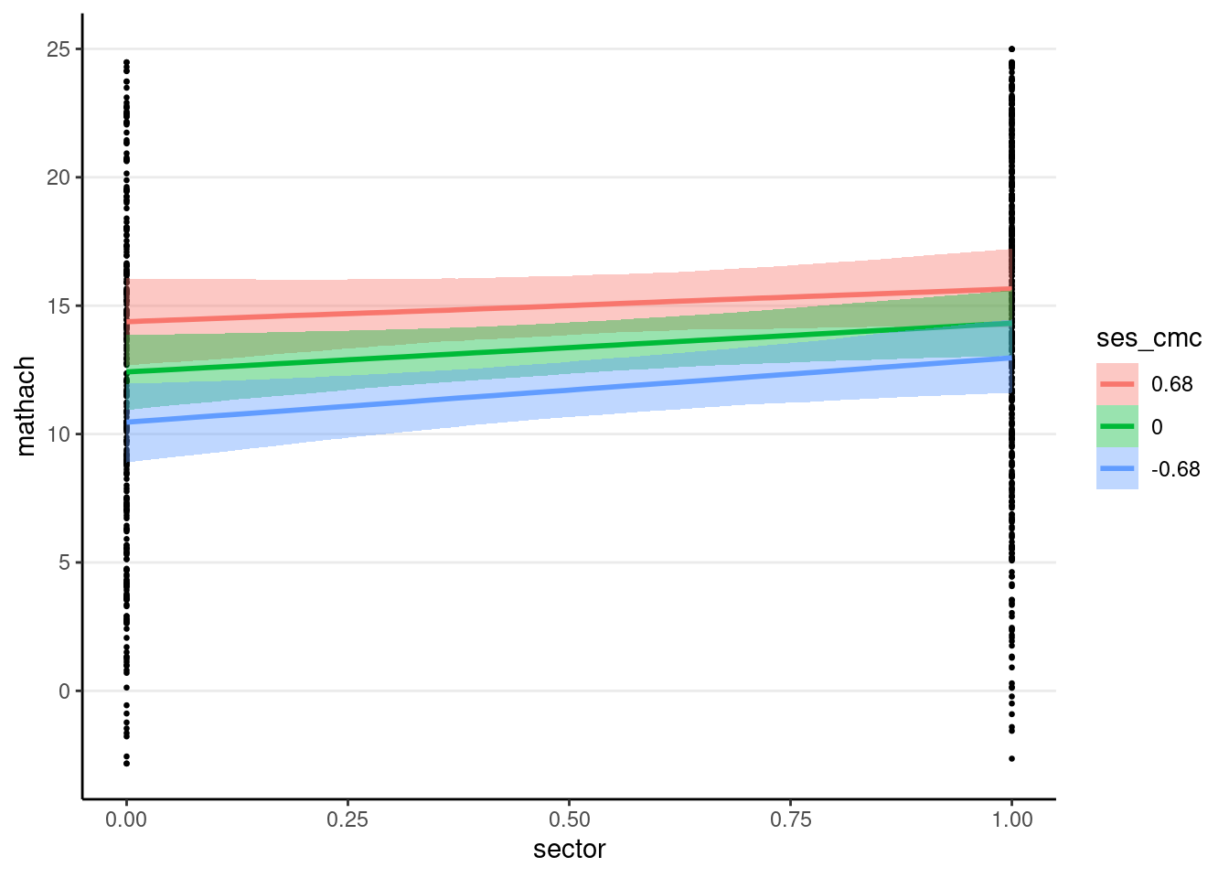
Plotting
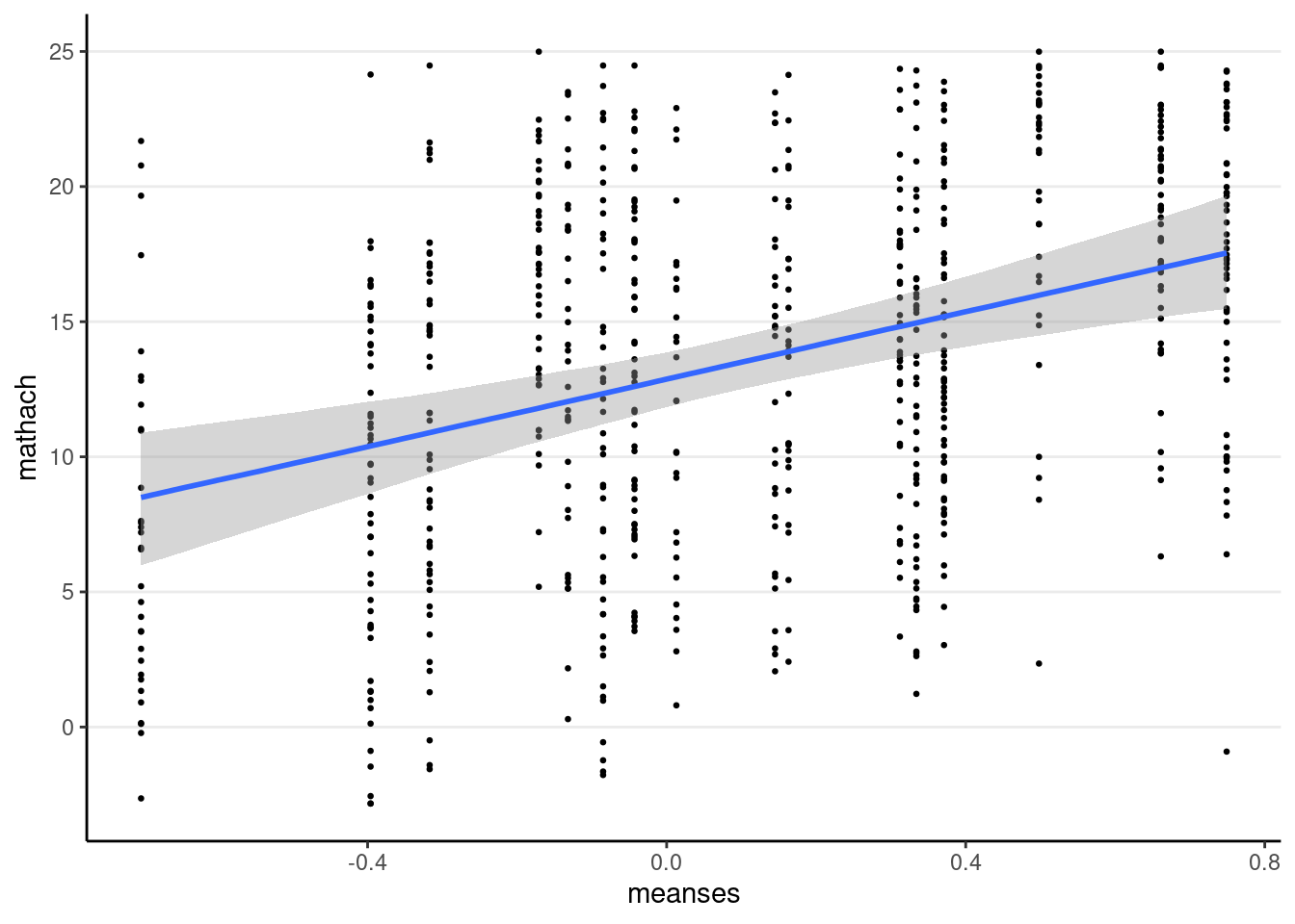
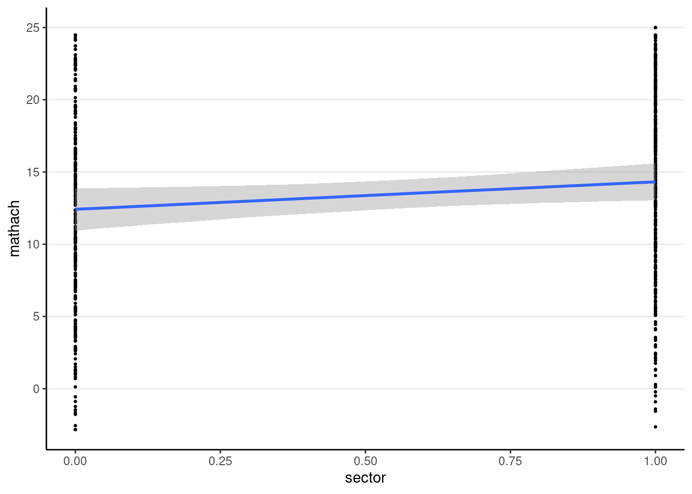
You can use the conditional_effects() function
plot(
    conditional_effects(crlv_int_brm),
    points = TRUE,  # show data
    point_args = list(size = 0.5)  # make points smaller
)
The sjPlot::plot_model() function also works; you can try it yourself.
Tables
modelsummary::msummary() also works; for now, however, you’ll need to get the intervals instead of the standard errors in the table.
msummary(list("Bayesian" = crlv_int_brm),
         estimate = "{estimate} [{conf.low}, {conf.high}]",
         statistic = NULL)
># Warning:
># `modelsummary` uses the `performance` package to extract goodness-of-fit
># statistics from models of this class. You can specify the statistics you wish
># to compute by supplying a `metrics` argument to `modelsummary`, which will then
># push it forward to `performance`. Acceptable values are: "all", "common",
># "none", or a character vector of metrics names. For example: `modelsummary(mod,
># metrics = c("RMSE", "R2")` Note that some metrics are computationally
># expensive. See `?performance::performance` for details.
># This warning appears once per session.| Bayesian | |
|---|---|
| b_Intercept | 11.769 [10.271, 13.199] |
| b_meanses | 6.261 [3.475, 9.122] |
| b_sector | 1.899 [−0.026, 3.888] |
| b_ses_cmc | 2.869 [1.814, 3.843] |
| b_sector × ses_cmc | −0.906 [−2.257, 0.592] |
| sd_id__Intercept | 1.621 [0.950, 2.807] |
| sd_id__ses_cmc | 0.465 [0.022, 1.538] |
| cor_id__Intercept__ses_cmc | 0.268 [−0.882, 0.961] |
| sigma | 5.707 [5.420, 6.030] |
| Num.Obs. | 686 |
| R2 | 0.270 |
| R2 Adj. | 0.241 |
| R2 Marg. | 0.241 |
| ELPD | −2177.4 |
| ELPD s.e. | 15.9 |
| LOOIC | 4354.8 |
| LOOIC s.e. | 31.8 |
| WAIC | 4354.7 |
| RMSE | 5.63 |
| r2.adjusted.marginal | 0.178 |
Bonus: More on Maximum Likelihood
If you are a stat/quant major or are interested in the math, then you should study the equation a little bit.
The mixed model can be written in matrix form. Let \(\bv y_j = [\bv y_1, \bv y_2, \ldots, \bv y_J]^\top\) be the column vector of length \(N\) for the outcome variable, \(\bv X\) be the \(N \times p\) predictor matrix (with the first column as the intercept), and \(\bv Z\) be the \(N \times Jq\) design matrix for the random effects with \(q\) being the number of random coefficients. To make things more concrete, if we have the model
\(\bv y\) is the outcome mathach
matrix(head(getME(m1, "y")))># [,1]
># [1,] 5.876
># [2,] 19.708
># [3,] 20.349
># [4,] 8.781
># [5,] 17.898
># [6,] 4.583\(\bv X\) is a \(N \times 3\) matrix, with the first column containing all 1s (for the intercept), the second column is meanses, and the third column is ses
head(getME(m1, "X"))># (Intercept) meanses ses
># 1 1 -0.428 -1.528
># 2 1 -0.428 -0.588
># 3 1 -0.428 -0.528
># 4 1 -0.428 -0.668
># 5 1 -0.428 -0.158
># 6 1 -0.428 0.022And \(\bv Z\) is a block-diagonal matrix \(\mathrm{diag}[\bv Z_1, \bv Z_2, \ldots, \bv Z_J]\), where each \(\bv Z_j\) is an \(n_j \times 2\) matrix with the first column containing all 1s and the second column containing the ses variable for cluster \(j\)
dim(getME(m1, "Z"))># [1] 7185 320# Show the first two blocks
getME(m1, "Z")[1:72, 1:4]># 72 x 4 sparse Matrix of class "dgCMatrix"
># 1224 1224 1288 1288
># 1 1 -1.528 . .
># 2 1 -0.588 . .
># 3 1 -0.528 . .
># 4 1 -0.668 . .
># 5 1 -0.158 . .
># 6 1 0.022 . .
># 7 1 -0.618 . .
># 8 1 -0.998 . .
># 9 1 -0.888 . .
># 10 1 -0.458 . .
># 11 1 -1.448 . .
># 12 1 -0.658 . .
># 13 1 -0.468 . .
># 14 1 -0.988 . .
># 15 1 0.332 . .
># 16 1 -0.678 . .
># 17 1 -0.298 . .
># 18 1 -1.528 . .
># 19 1 0.042 . .
># 20 1 -0.078 . .
># 21 1 0.062 . .
># 22 1 -0.128 . .
># 23 1 0.472 . .
># 24 1 -0.468 . .
># 25 1 -1.248 . .
># 26 1 -0.628 . .
># 27 1 0.832 . .
># 28 1 -0.568 . .
># 29 1 -0.258 . .
># 30 1 -0.138 . .
># 31 1 -0.478 . .
># 32 1 -0.948 . .
># 33 1 0.282 . .
># 34 1 -0.118 . .
># 35 1 -0.878 . .
># 36 1 -0.938 . .
># 37 1 -0.548 . .
># 38 1 0.142 . .
># 39 1 0.972 . .
># 40 1 0.372 . .
># 41 1 -1.658 . .
># 42 1 -1.068 . .
># 43 1 -0.248 . .
># 44 1 -1.398 . .
># 45 1 0.752 . .
># 46 1 0.012 . .
># 47 1 -0.418 . .
># 48 . . 1 -0.788
># 49 . . 1 -0.328
># 50 . . 1 0.472
># 51 . . 1 0.352
># 52 . . 1 -1.468
># 53 . . 1 0.202
># 54 . . 1 -0.518
># 55 . . 1 -0.158
># 56 . . 1 0.042
># 57 . . 1 0.682
># 58 . . 1 1.262
># 59 . . 1 0.152
># 60 . . 1 -0.678
># 61 . . 1 0.332
># 62 . . 1 -0.728
># 63 . . 1 1.262
># 64 . . 1 0.612
># 65 . . 1 0.692
># 66 . . 1 1.082
># 67 . . 1 0.222
># 68 . . 1 0.032
># 69 . . 1 -0.118
># 70 . . 1 -0.488
># 71 . . 1 0.322
># 72 . . 1 0.592The matrix form of the model is \[\bv y = \bv X \bv \gamma + \bv Z \bv u + \bv e,\] with \(\bv \gamma\) being a \(N \times p\) vector of fixed effects, \(\bv \tau\) a vector of random effect variances, \(\sigma\) the level-1 error term, \(\bv u\) containing the \(u_0\) and \(u_1\) values for all clusters (320 in total), and \(\bv e\) containing the level-1 errors. The distributional assumptions are \(\bv u_j \sim N_2(\bv 0, \bv G)\) and \(e_{ij} \sim N(0, \sigma)\).
The marginal distribution of \(\bv y\) is thus \[\bv y \sim N_p\left(\bv X \bv \gamma, \bv V(\bv \tau, \sigma)\right),\] where \(\bv V(\bv \tau, \sigma) = \bv Z \bv G \bv Z^\top + \sigma^2 \bv I\) with \(\bv I\) being an \(N \times N\) identity matrix.
The log-likelihood function for a multilevel model is \[\ell(\bv \gamma, \bv \tau, \sigma; \bv y) = - \frac{1}{2} \left\{\log | \bv V(\bv \tau, \sigma)| + (\bv y - \bv X \bv \gamma)^\top \bv V^{-1}(\bv \tau, \sigma) (\bv y - \bv X \bv \gamma) \right\} + K\] with \(K\) not involving the model parameters. Check out this paper if you want to learn more about the log-likelihood function used in lme4.
Note: When statistician says log, it means the natural logarithm, i.e., log with base e (sometimes written as ln)
Standard Errors
For the fixed effects, the sampling variance has the analytic form
\[(\bv X^\top \bv V^{-1} \bv X)^{-1}\]
# Asympotitc standard error (ASE) from lme4
vcov(m_lv2)
># 2 x 2 Matrix of class "dpoMatrix"
># (Intercept) meanses
># (Intercept) 0.0222845612 -0.0002358047
># meanses -0.0002358047 0.1306518973# ASE using formula
ase <- function(X = cbind(1, m_lv2@frame$meanses),
V = V_m_lv2) {
solve(crossprod(X, solve(V, X)))
}
ase() # the results are identical># 2 x 2 Matrix of class "dgeMatrix"
># [,1] [,2]
># [1,] 0.0222845612 -0.0002358047
># [2,] -0.0002358047 0.1306518973