Week 11 (R): Causal Inference

Load Packages and Import Data

# To install a package, run the following ONCE (and only once on your computer)
# install.packages("psych")
library(here)  # makes reading data more consistent
library(tidyverse)  # for data manipulation and plotting
library(haven)  # for importing SPSS/SAS/Stata data
library(dagitty)  # for DAG
library(ggdag)  # for DAG in ggplot style
library(lme4)  # for multilevel analysis
library(sjPlot)  # for plotting
library(mediation)  # for plotting
library(modelsummary)  # for making tables

Causal Diagram

You can use the daggity package to draw causal diagrams, specifically directed acyclic graphs (DAGs). The ggdag package further makes the DAG in ggplot style. The following shows a confounder C.

dag1 <- dagitty(
    "dag{
      X -> Y; C -> X; C -> Y
    }"
)
coordinates(dag1) <- list(x = c(X = 0, C = 1, Y = 2),
                          y = c(X = 0, C = 1, Y = 0))
# Plot
ggdag(dag1) + theme_dag()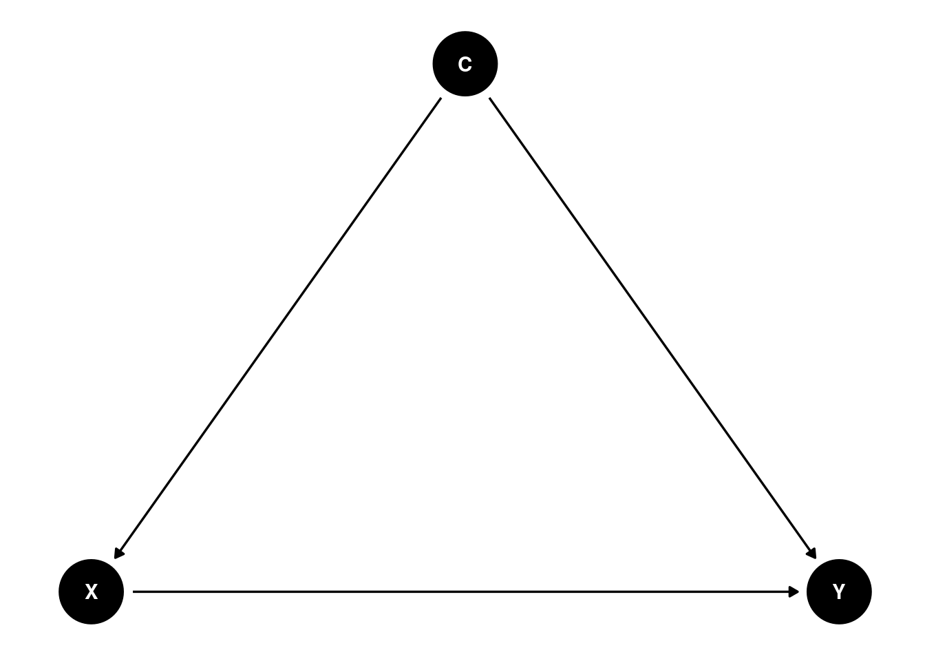

The dagitty package is very powerful, as it can inform what covariates need to be adjusted for a given causal diagram. This requires strong assumptions on the causal structure of the data. For example,

adjustmentSets(dag1, exposure = "X", outcome = "Y",
               effect = "direct")

># { C }

tells you that C needs to be adjusted to obtain a causal effect of X to Y.

Statistical Adjustment

Import Data

# Import HSB data
hsball <- read_sav(here("data_files", "hsball.sav"))
# Cluster means
hsball <- hsball %>%
    group_by(id) %>%   # operate within schools
    mutate(ses_cm = mean(ses),
           minority_cm = mean(minority)) %>%
    ungroup()

Unadjusted and Adjusted Models

The observed difference between the two types of schools is not the causal effect of sector, namely,

What would the students perform if they changed from a public school to a Catholic school

when students can “select” to attend different schools. However, if we can obtain a complete set of variables that unconfounds the X → Y path, the adjusted coefficient can be interpreted as causal effects.

Assumptions:

• The covariates used completely unconfound all confounding paths
• The covariates used do not contain mediators or colliders
• All standard assumptions in regression and multilevel models (e.g., linearity)

Let’s say we think that the path is confounded because students with certain SES backgrounds may be more likely to go into public schools than Catholic schools. Also, minority students may be more likely to go to public schools. Both ses and minority are also on a causal path to mathach, and so both are on confounding paths of sector → mathach.

# Unadjusted model
m_unadjusted <- lmer(mathach ~ sector + (1 | id), data = hsball)
# Adjusted model (with ses and minority)
m_adjusted <- lmer(mathach ~ sector + ses_cm + minority_cm +
                       ses + minority + (ses + minority | id),
                   data = hsball)
msummary(list(unadjusted = m_unadjusted,
              adjusted = m_adjusted))

	unadjusted	adjusted
(Intercept)	11.393	12.682
	(0.293)	(0.213)
sector	2.805	1.545
	(0.439)	(0.303)
ses_cm		2.521
		(0.431)
minority_cm		0.096
		(0.598)
ses		1.936
		(0.118)
minority		−2.945
		(0.251)
SD (Intercept id)	2.584	1.372
SD (ses id)		0.554
SD (minority id)		1.195
Cor (Intercept~ses id)		0.198
Cor (Intercept~minority id)		−0.053
Cor (ses~minority id)		−0.989
SD (Observations)	6.257	5.981
Num.Obs.	7185	7185
R2 Marg.	0.041	0.209
R2 Cond.	0.181	0.261
AIC	47088.1	46375.3
BIC	47115.7	46464.7
ICC	0.1	0.07
RMSE	6.20	5.92

The estimated coefficient is smaller for the adjusted model. Note that this is only an example; it is unlikely that these two variables are sufficient to unconfound the associations between sector and mathach. For example, non-public schools may admit only students who already have a good math background, so we would need to adjust for a measure of math ability or aptitude.

Berkeley Admission Example

It is a famous data set, which is available in base R by calling

UCBAdmissions

># , , Dept = A
># 
>#           Gender
># Admit      Male Female
>#   Admitted  512     89
>#   Rejected  313     19
># 
># , , Dept = B
># 
>#           Gender
># Admit      Male Female
>#   Admitted  353     17
>#   Rejected  207      8
># 
># , , Dept = C
># 
>#           Gender
># Admit      Male Female
>#   Admitted  120    202
>#   Rejected  205    391
># 
># , , Dept = D
># 
>#           Gender
># Admit      Male Female
>#   Admitted  138    131
>#   Rejected  279    244
># 
># , , Dept = E
># 
>#           Gender
># Admit      Male Female
>#   Admitted   53     94
>#   Rejected  138    299
># 
># , , Dept = F
># 
>#           Gender
># Admit      Male Female
>#   Admitted   22     24
>#   Rejected  351    317

# ?UCBAdmissions  # see documentation

The data, however, is a three-dimension contingency table, which cannot be directly analyzed by regression/multilevel models. Here we convert the data to a data frame:

berkeley_admit <- UCBAdmissions %>%
    # to data frame
    as.data.frame() %>%
    # one column for admit and one for reject
    pivot_wider(names_from = Admit, values_from = Freq)
berkeley_admit

ABCDEFGHIJ0123456789

Gender <fct>	Dept <fct>	Admitted <dbl>	Rejected <dbl>
Male	A	512	313
Female	A	89	19
Male	B	353	207
Female	B	17	8
Male	C	120	205
Female	C	202	391
Male	D	138	279
Female	D	131	244
Male	E	53	138
Female	E	94	299

Next

12

Previous

1-10 of 12 rows

The outcome is the number of people admitted, which can be modelled as a binomial variable (i.e., number of “successes” out of a known total). We will talk about generalized linear models and generalized linear mixed models in a future week, but here’s the syntax when we ignore the department and just look at the overall success rate across Gender:

# For binomial, the outcome has the syntax `cbind(# successes, # failures)`
m_single <- glm(
    cbind(Admitted, Rejected) ~ Gender,
    data = berkeley_admit,
    # specify family
    family = binomial("logit")
)
summary(m_single)

># 
># Call:
># glm(formula = cbind(Admitted, Rejected) ~ Gender, family = binomial("logit"), 
>#     data = berkeley_admit)
># 
># Deviance Residuals: 
>#      Min        1Q    Median        3Q       Max  
># -16.7915   -4.7613   -0.4365    5.1025   11.2022  
># 
># Coefficients:
>#              Estimate Std. Error z value Pr(>|z|)    
># (Intercept)  -0.22013    0.03879  -5.675 1.38e-08 ***
># GenderFemale -0.61035    0.06389  -9.553  < 2e-16 ***
># ---
># Signif. codes:  0 '***' 0.001 '**' 0.01 '*' 0.05 '.' 0.1 ' ' 1
># 
># (Dispersion parameter for binomial family taken to be 1)
># 
>#     Null deviance: 877.06  on 11  degrees of freedom
># Residual deviance: 783.61  on 10  degrees of freedom
># AIC: 856.55
># 
># Number of Fisher Scoring iterations: 4

plot_model(m_single, type = "pred")

># $Gender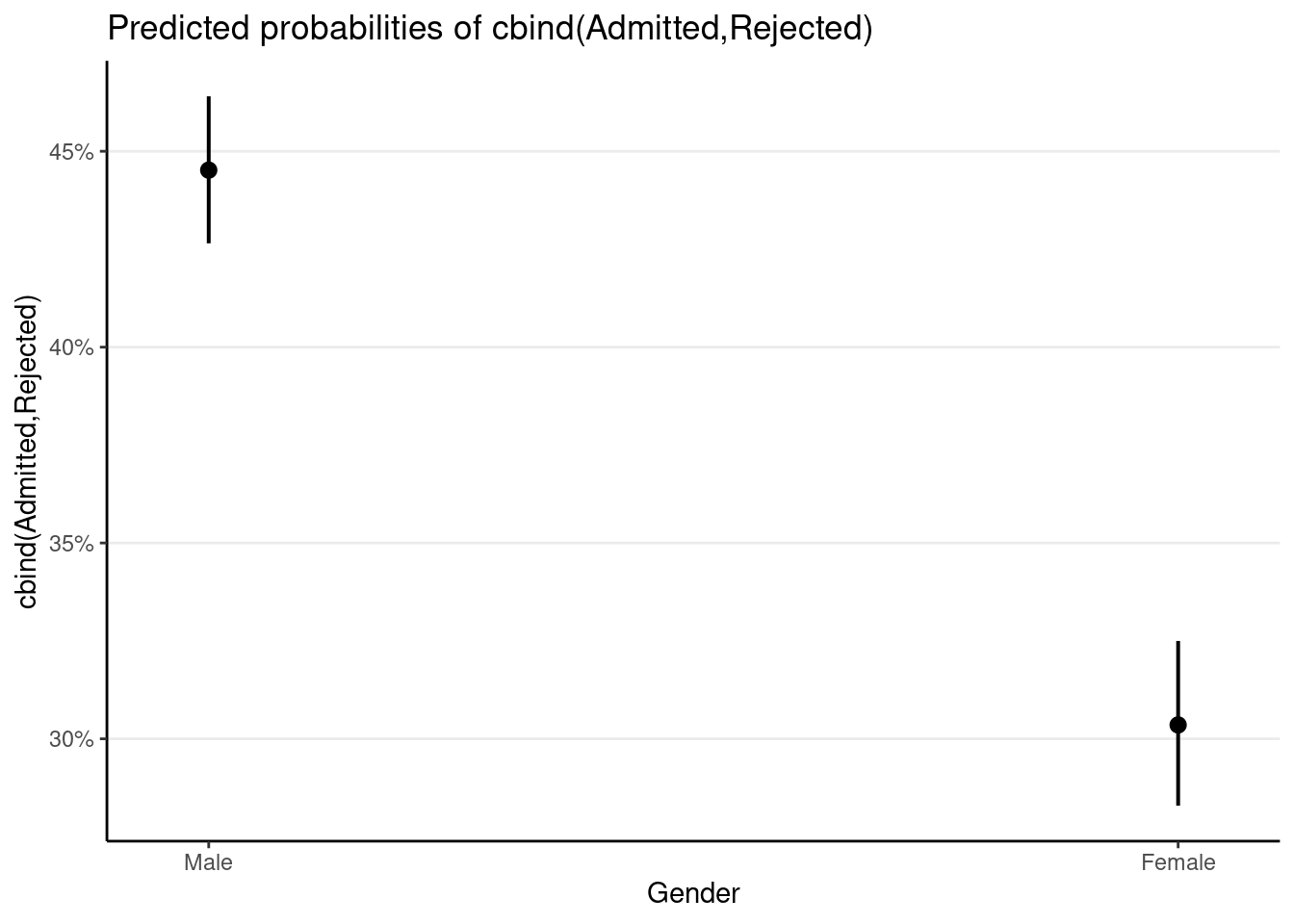

which shows a lower admission rate for females. However, if we also consider the department in a multilevel model, which also requires accounting for the proportion of female applicants in a given department, we have

# Cluster mean for Gender
berkeley_admit <- berkeley_admit |>
    group_by(Dept) |>
    mutate(
        # Proportion of female applicants
        Gender_cm = sum(Admitted[2], Rejected[2]) /
            sum(Admitted, Rejected)) |>
    ungroup()
berkeley_admit

ABCDEFGHIJ0123456789

Gender <fct>	Dept <fct>	Admitted <dbl>	Rejected <dbl>	Gender_cm <dbl>
Male	A	512	313	0.11575563
Female	A	89	19	0.11575563
Male	B	353	207	0.04273504
Female	B	17	8	0.04273504
Male	C	120	205	0.64596950
Female	C	202	391	0.64596950
Male	D	138	279	0.47348485
Female	D	131	244	0.47348485
Male	E	53	138	0.67294521
Female	E	94	299	0.67294521

Next

12

Previous

1-10 of 12 rows

# Use `glmer()` for non-normal outcomes
m_mlm <- glmer(
    cbind(Admitted, Rejected) ~ Gender + Gender_cm + (Gender | Dept),
    data = berkeley_admit,
    # specify family
    family = binomial("logit")
)
summary(m_mlm)

># Generalized linear mixed model fit by maximum likelihood (Laplace
>#   Approximation) [glmerMod]
>#  Family: binomial  ( logit )
># Formula: cbind(Admitted, Rejected) ~ Gender + Gender_cm + (Gender | Dept)
>#    Data: berkeley_admit
># 
>#      AIC      BIC   logLik deviance df.resid 
>#    127.7    130.7    -57.9    115.7        6 
># 
># Scaled residuals: 
>#      Min       1Q   Median       3Q      Max 
># -0.32605 -0.21671 -0.03468  0.14024  1.19665 
># 
># Random effects:
>#  Groups Name         Variance Std.Dev. Corr 
>#  Dept   (Intercept)  0.7428   0.8619        
>#         GenderFemale 0.1131   0.3363   -0.14
># Number of obs: 12, groups:  Dept, 6
># 
># Fixed effects:
>#              Estimate Std. Error z value Pr(>|z|)
># (Intercept)    0.6132     1.0576   0.580    0.562
># GenderFemale   0.1685     0.1722   0.978    0.328
># Gender_cm     -3.1551     2.5040  -1.260    0.208
># 
># Correlation of Fixed Effects:
>#             (Intr) GndrFm
># GenderFemal  0.115       
># Gender_cm   -0.942 -0.181

plot_model(m_mlm, terms = c("Dept [A, B, C, D, E, F]", "Gender"),
           type = "pred", pred.type = "re")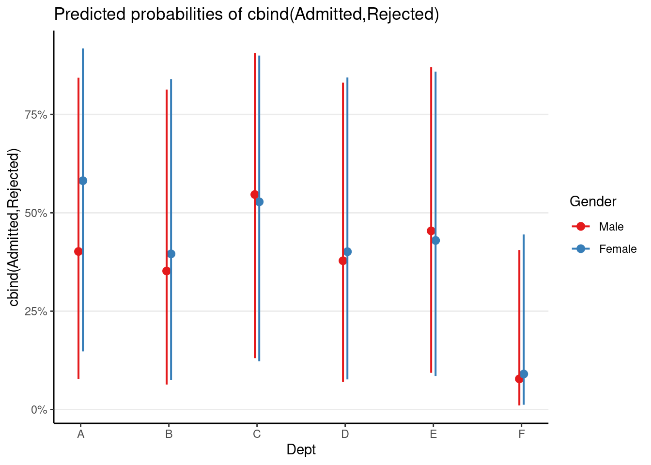

As can be seen, there was insufficient evidence for gender bias at the within-department level.

Bonus: Mediation

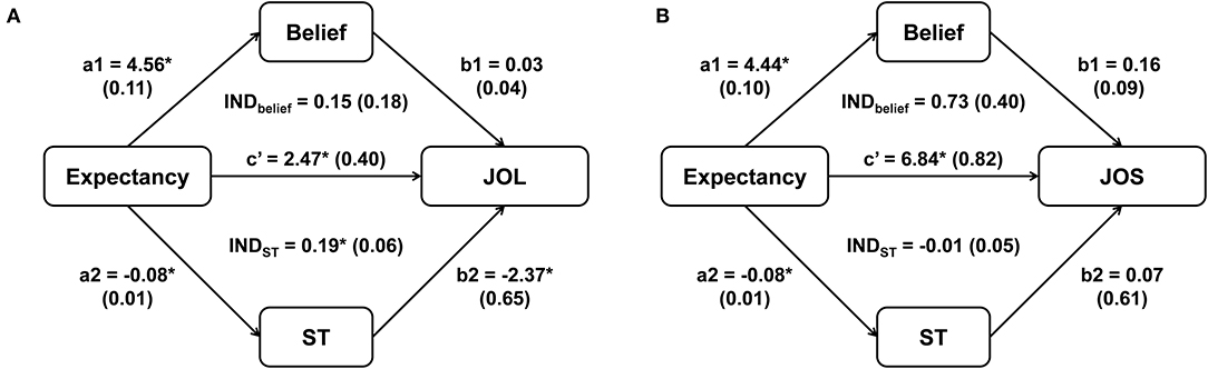
Here’s one of the examples from this paper (https://doi.org/10.3389/fpsyg.2020.00637), which reanalyzed some previous data on how beliefs influence judgments of learning (JOL) from Experiment 1 of Schaper et al. (2019). The mediation model here is Expectancy → ST (self-paced study time in seconds) → JOL. See this figure from the paper: https://www.frontiersin.org/files/Articles/522445/fpsyg-11-00637-HTML/image_m/fpsyg-11-00637-g002.jpg (the upper part).

Generally speaking, a mediation model has two components: (a) treatment to mediator, and (b) mediator to outcome, while holding the treatment constant. We can fit separate models to each component.

Import Data

dat <- haven::read_sav("https://osf.io/kewdc/download")
head(dat)

ABCDEFGHIJ0123456789

sub <dbl>	expectancy <dbl>	diffbelief <dbl>	jol <dbl>	st_original <dbl>	st_log <dbl>
1	-1	-10	70	9641	9.173780
1	-1	-10	80	3894	8.267192
1	-1	-10	100	15223	9.630563
1	-1	-10	70	6989	8.852093
1	-1	-10	90	15950	9.677214
1	-1	-10	70	14752	9.599134

6 rows | 1-6 of 13 columns

dat$jol10 <- dat$jol / 10  # rescale JOL from 0-100 to 0-10
dat$belief10 <- dat$belief / 10  # rescale belief from 0-100 to 0-10

Treatment → Mediator

Here the treatment is at level 1, and effect coding was used (-1 for control, 1 for treatment). With effect coding, the treatment coefficient is interpreted as the difference between a condition and the average, because one unit difference in the treatment variable means going from -1 to 0, where 0 is the average of the two conditions.

# Component (a). Cannot include random slope term in `lme4`
# with two observations per cluster. Can try glmmTMB(..., disp = ~0)
ma <- lmer(belief10 ~ expectancy + (1 | sub), data = dat)
plot_model(ma, type = "pred")

># $expectancy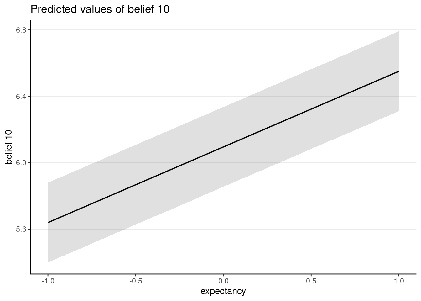

Mediator → Outcome, Holding Treatment Constant

Because the mediator has a cluster mean component, we should also include it.

dat <- dat |>
    group_by(sub) |>
    mutate(belief10_pm = mean(belief10)) |>
    ungroup()

# Component (b). Make sure to include the treatment variable.
mb <- lmer(jol10 ~ belief10 + belief10_pm + expectancy +
               (belief10 | sub), data = dat)
plot_model(mb, type = "pred", terms = "belief10")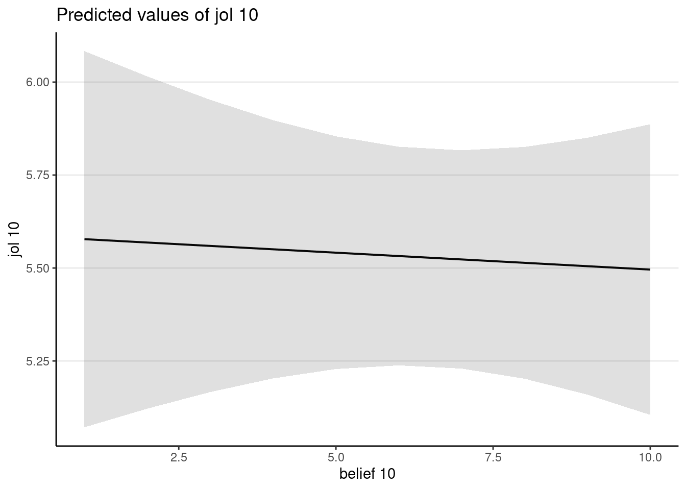

The mediator does not have a strong direct effect on the outcome.

Mediation Analysis

You should only perform a mediation analysis when the data support the causal directions of the variables, or when you are willing to make strong causal assumptions. You can use the mediation::mediate() function.

# Input: components (a) and (b). This takes a few minutes because
# it uses simulations.
m_med <- mediate(
    ma,
    model.y = mb,
    treat = "expectancy",  # name of mediator
    mediator = "belief10",  # name of mediator
    control.value = -1,
    treat.value = 1
)
summary(m_med)

># 
># Causal Mediation Analysis 
># 
># Quasi-Bayesian Confidence Intervals
># 
># Mediator Groups: sub 
># 
># Outcome Groups: sub 
># 
># Output Based on Overall Averages Across Groups 
># 
>#                Estimate 95% CI Lower 95% CI Upper p-value    
># ACME            -0.0056      -0.0878         0.07    0.88    
># ADE              0.5677       0.4536         0.67  <2e-16 ***
># Total Effect     0.5621       0.4606         0.67  <2e-16 ***
># Prop. Mediated  -0.0097      -0.1658         0.12    0.88    
># ---
># Signif. codes:  0 '***' 0.001 '**' 0.01 '*' 0.05 '.' 0.1 ' ' 1
># 
># Sample Size Used: 7680 
># 
># 
># Simulations: 1000

plot(m_med)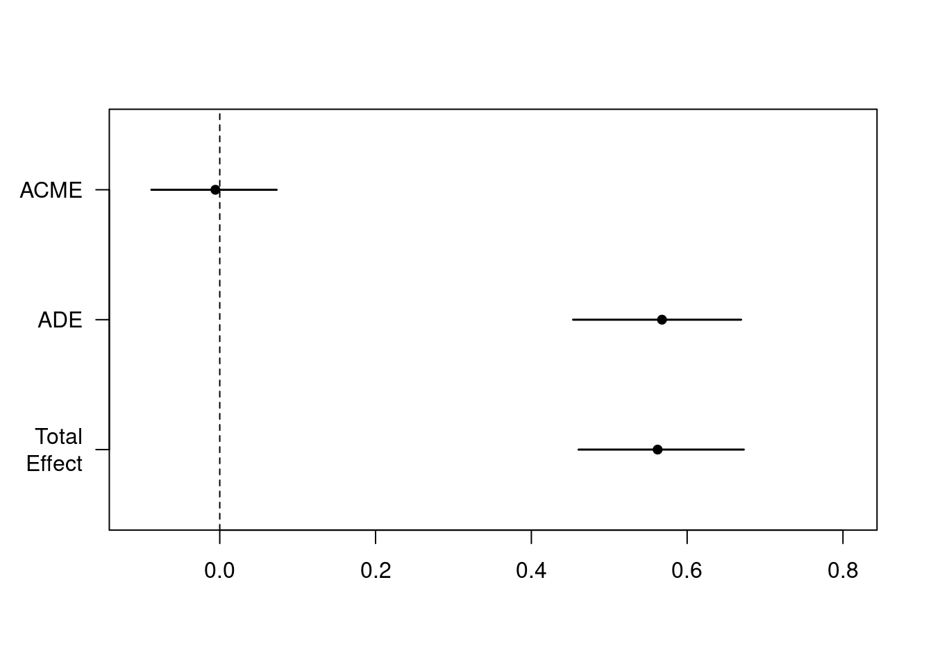

The row labeled ACME is the estimated mediation effect, which is not statistically significant in this example.